1. mcg: McGeoch's method for signal sequence recognition
2. gvh: von Heijne's method for signal sequence recognition.
3. lip: von Heijne's Signal Peptidase II consensus sequence score. Binary attribute.
4. chg: Presence of charge on N-terminus of predicted lipoproteins. Binary attribute.
5. aac: score of discriminant analysis of the amino acid content of outer membrane and periplasmic proteins.
6. alm1: score of the ALOM membrane spanning region prediction program.
7. alm2: score of ALOM program after excluding putative cleavable signal regions from the sequence.

Output attributes are:

1. cp (cytoplasm)
2. im (inner membrane without signal sequence)
3. pp (perisplasm)
4. imU (inner membrane, uncleavable signal sequence)
5. om (outer membrane)
6. omL (outer membrane lipoprotein)
7. imL (inner membrane lipoprotein)
8. imS (inner membrane, cleavable signal sequence)

1. Normalize the data
2. Create a Neuroph project
3. Creating a Training Set
4. Create a neural network
5. Train the network
6. Test the network to make sure that it is trained properly

In this experiment we will demonstrate the use of some standard and advanced training techniques. Several architectures will be tried out, based on which we will be able to determine what brings us the best results for our problem.

 B = (A - min(A)) / (max(A) - min(A)) * ( D - C ) + C

Where B is the standardized value, and D and C determine the range in which we want our value to be, in this case C= 1 and D = 0.

Normalized values are saved in data.txt file because they will be used for training and testing neural network

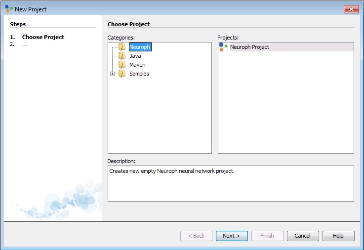
We create a new project in Neuroph Studio by clicking File > New Project, then we choose Neuroph project and click 'Next' button.

In a new window we define project name and location. After that we click 'Finish' and a new project is created and will appear in projects window, on the left side of Neuroph Studio.

As supervised training proceeds, the neural network is taken through a number of iterations, until the output of the neural network matches the anticipated output, with a reasonably small rate of the error.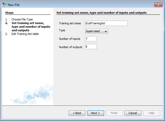

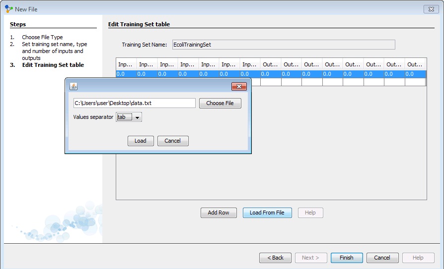
After clicking 'Next' we need to insert data into training set table. All data could be inserted manually, but we have a large number of data instances and it would be a lot more easier to load all data directly from some file. We click on 'Choose File' and select file in which we saved our normalized data set. Values in that file are separated by tab.

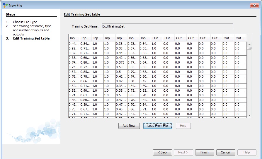
Then, we click 'Load' and all data will be loaded into table. We can see that this table has 15 columns, first 7 of them represents inputs, and last 8 of them represents outputs from our data set.

After clicking 'Finish' new training set will appear in our project.
To be able to decide which is the best solution for our problem we will create several neural networks, with different sets of parameters, and most of them will be based on this training set.

Standard approaches to validation of neural networks are mostly based on empirical evaluation through simulation and/or experimental testing. There are several methods for supervised training of neural networks. The backpropagation algorithm is the most commonly used training method for artificial neural networks.

Backpropagation is a supervised learning method. It requires a data set of the desired output for many inputs, making up the training set. It is most useful for feed-forward networks (networks that have no feedback, or simply, that have no connections that loop). Main idea is to distribute the error function across the hidden layers, corresponding to their effect on the output.

A multilayer perceptron is a feedforward artificial neural network model that maps sets of input data onto a set of appropriate output. It consists of multiple layers of nodes in a directed graph, with each layer fully connected to the next one. Except for the input nodes, each node is a neuron with nonlinear activation function Multylauer perceptron utilizes a supervised learning technique called backpropagation for training the network. It is a modification of the standard linear perceptron, which can distinguish data that is not linearly separable.

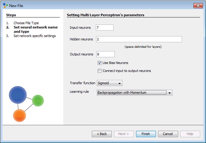
In the next window we will set multy layer perceptron's parameters. The number of input and output neurons are the same as in the training set. And now we have to choose number of hidden layers, and number of neurons in each layer.

Problems that require more than one hidden layers are rarely encountered. For many practical problems, there is no reason to use any more than one hidden layer. One layer can approximate any function that contains a continuous mapping from one finite space to another. Deciding the number of hidden neuron layers is only a small part of the problem. We must also determine how many neurons will be in each of these hidden layers. Both the number of hidden layers and the number of neurons in each of these hidden layers must be carefully considered.

Using too few neurons in the hidden layers will result in something called underfitting. Underfitting occurs when there are too few neurons in the hidden layers to adequately detect the signals in a complicated data set.

Using too many neurons in the hidden layers can result in several problems. First, too many neurons in the hidden layers may result in overfitting. Overfitting occurs when the neural network has so much information processing capacity that the limited amount of information contained in the training set is not enough to train all of the neurons in the hidden layers. A second problem can occur even when the training data is sufficient. An inordinately large number of neurons in the hidden layers can increase the time it takes to train the network. The amount of training time can increase to the point that it is impossible to adequately train the neural network.

Obviously, some compromise must be reached between too many and too few neurons in the hidden layers.

We have decided to have 1 layer and 2 hidden neurons in this first training attempt. Than we check 'Use Bias Neurons' option and choose 'Sigmond' for transfer function (because our data set is normalized). For learning rule we choose 'Backpropagation with Momentum'. The momentum is added to speed up the process of learning and to improve the efficiency of the algorithm.

Bias neuron is very important, and the error-back propagation neural network without Bias neuron for hidden layer does not learn. The Bias weights control shapes, orientation and steepness of all types of Sigmoidal functions through data mapping space. A bias input always has the value of 1. Without a bias, if all inputs are 0, the only output ever possible will be a zero.

Next, we click 'Finish' and the first neural network is created. In the picture below we can see the graph view of this neural network.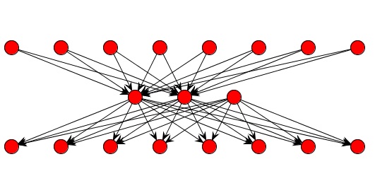

Figure shows the input, the output and hidden neurons and how they are connected with each other. Except for two neurons with activation level 1 (bias activation), all other neurons have an activation level 0. These two neurons represent bias neurons, as we explained above.

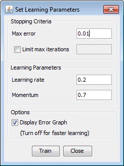
After we have created training set and neural network we can train neural network. First, we select training set, click 'Train', and then we have to set learning parameters for training.

Learning rate is a control parameter of training algorithms, which controls the step size when weights are iteratively adjusted.

To help avoid settling into a local minimum, a momentum rate allows the network to potentially skip through local minima. A momentum rate set at the maximum of 1.0 may result in training which is highly unstable and thus may not achieve even a local minima, or the network may take an inordinate amount of training time. If set at a low of 0.0, momentum is not considered and the network is more likely to settle into a local minimum.

When the Total Net Error value drops below the max error, the training is complete. If the error is smaller we get a better approximation.

Now, click 'Train' button and see what happens.

We can see in pictures below that training was unsuccesfull. After 10008 iterations Neural Network failed to learn problem with error less than 0,01. We can test this network but error will be greater than expected.

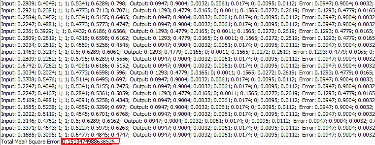
Step 6.1. Testing the Neural Network

After the network is trained, we click 'Test', in order to see the total error, and all the individual errors. The result show us  that total mean square error is  aproximatly 0.13, which is to much. Individual errors are also pretty big. Lets look at last result. Values of output are 0.9781, 0.0193, 0.0035, 0 0.0239. 0.0108, 0 and -0.9932 but result should be 0,0,0,0,0,0,0,1. With this information we can conclude that this Neural Network is not good enough.

Step 5.2. Train the network

So let us try something else. We will update the weight of learning rate and increase it . In network window click Randomize button and then click Train button. That means that we will set value of 0.2 in learning rate label replace with a new value 0.3 and click 'Train' button.

After training Network with these parameters we got better results but still not good enough.

Increasing the value of learning rate we conclude that the objective error function oscillates more and the network reaches a state where no useful training takes place.

In the table below for the next three sessions we will present the results of other trainings for the first architecture. For other trainings is not given graphic.

Table 1. Training results for the first architecture

Based on data from Table 1it can be seen that regardless of the parameters of training error do not falls below a specified level, even if we train the network through a different number of iterations. This may be due to the small number of hidden neurons. In the following solution we will increase the number of hidden neurons.

Step 4.5. Create a Neural Network

Next Neural Network will have same number of input and output neurons but different number of neurons in hidden layer. We will use 4 hidden layer neurons. Network in named NN4.

Step 5.5. Train the network

First training course, of second architecture, we will start with extremely low values of learning rate and momentum. First click on button 'Train'. In 'Set Learning parameters' dialog, field 'set Stopping criteria enter 0.01 as max error. In order to graphically display, the training of this network, was clearer. In field 'set Learning parameters', enter 0.01 for 'Learning rate' and 0.05 for 'Momentum'. After entering this values click on button 'Train'.

During the testing we unsuccessfully trained the neural network named NN4. The summary of the results are shown in the Table 2.

Total Net Error is still higher than set value.

From the graphics above can be seen from iteration to iteration there are no large shifts in the prediction. More accurate in predicting, fluctuations are very small and the values are around 0.1. Reason for such a small fluctuation is that the learning rate is very close to zero. Also because of such a small coefficient, of the learning rate, neural network has no the ability to learn quickly. On the other hand small value of momentum slows down the training of the system.

Step 5.6. Train the network

Like in last attempt we will try extremely high values of learning rate and momentum. Compared to previous training, we will just replace the values of learning rate and momentum. For learning rate we will enter 0.9 and for momentum also 0.9. Other options will be the same as in the previous training.

During the testing we unsuccessfully trained the neural network named NN4. The summary of the results are shown in the Table 2.

In picture below we see distinction between small values and large values of learning parameters. We set the momentum parameter too high and we have created a risk of overshooting the minimum, which caused the system to become unstable. On the other hand, the learning rate is very large, the weights diverge and the objective error function heavily oscillates and the network reaches a state where no useful training takes place.

Step 5.7. Train the network

In previous two attempts we used extreme values of learning parameters, so this time we will use recommended values. That is, 0.2 for learning rate and 0.7 for momentum.

Following useful conclusion can be drawn from this training. We can see that the architecture of four hidden neurons is not appropriate for this training set, because for continuing the training of the neural network we do not get the desired approximation of max error. Error is still much higher than desired level.

The oscillations are less than second training (which was expected because the parameters of training is less than in the previous case), but on the other side neural network has no the ability to learn quickly and the training of the system is slow (just like in first training).

In the table below for the previous three sessions we will present the results of all trainings for the second architecture.

Table 2. Training results for the second architecture

Total Net Errors

After several tries with different architecture and parameters we got results that are given in Table 3. There is interesting pattern in data. If we look number of hidden neurons and total net eror we can see that higher number of neurons leads us to lesser total net error.

Table 3. Training results for other architectures

Step 4.16. Create a Neural Network

This neural network will contain 20 neurons in hidden layer, as we see in picture below, and same options as previous networks.

Step 5.16. Train the network

First we will try with recommended values for learning rate and momentum. That is, 0.2 for learning rate and 0.7 for momenum.

During the testing we successfully trained the neural network named NN20. The summary of the results are shown at the final table at the end of this article.

The total net error slowly descends but with some oscilation and finally stops when reaches a level lower than a given (0.01) in 9306 iteration.

6.16. Test the network

Total Mean Square Error measures the average of the squares of the "errors". The error is the amount by which the value implied by the estimator differs from the quantity to be estimated. An mean square error of zero, meaning that the estimator predicts observations of the parameter with perfect accuracy, is the ideal, but is practically never possible. The unbiased model with the smallest mean square error is generally interpreted as best explaining the variability in the observations. The test showed that total mean square is 0.0354987642953988. The goal of experimental design is to construct experiments in such a way that when the observations are analyzed, the mean square error is close to zero relative to the magnitude of at least one of the estimated treatment effects.

Now we need to examine all the individual errors for every single instance and check if there are any extreme values. When you have a large data set, individual testing requires a lot of time. Instead of testing 336 observations we will random choose 5 observations which will be subjected to individual testing. Three following table will show the value of input, output and errors in 5 randomly selected observations. These values are taken from the window Test Results.

Table 4.1. Values of inputs

Table 4.2. Values of outputs

In introduction we mentioned that result can belong to one of three groups. So if protein localization site belongs to first group output would be 1, 0, 0,0,0,0,0,0 etc. After completion of testing would be ideal if the value of output after the test were the same as the output values before testing. As with other statistical methods, and classification using neural networks include errors that arise during the approximation. Individual error between the original and the assessed values are shown in Table 4.2.

For observation 221 and 225 we can say that there is reasonable mistake in classification. That is they are bigger than 1%. Therefor, we will continue training neural network by increasing learning rate to 0.3 (by 25%).

At the beginning we said that the goal is try to quickly find the smallest network that converges and then refine the answer by working back from there. Since we find the smallest neural network do the following:

• go back to the window of neural network,
• do not press the 'Reset' button,
• press the 'Train' button,
• value of learning rate increase by about 25%, so enter the value 0.3,
• again press 'Train' button,
• in network window press 'Test' button and you will see new test results.

When the training is complete, you will want to check the network performance. A learning neural network is expected to extract rules from a finite set of examples. It is often the case that the neural network memorizes the training data well, but fails to generate correct output for some of the new test data. Therefore, it is desirable to come up with some form of regularization.

One form of regularization is to split the training set into a new training set and a validation set. After each step through the new training set, the neural network is evaluated on the validation set. The network with the best performance on the validation set is then used for actual testing. Your new training set should consist of 80% - 90% of the original training set, and the remaining 10% - 20% would be classified in the validation set. Then you have to compute the validation error rate periodically during training and stop training when the validation error rate starts to go up. However, validation error is not a good estimate of the generalization error, if your initial set consists of a relatively small number of instances.

One way to get appropriate estimate of the generalization error is to run the neural network on the test set of data that is not used at all during the training process. The generalization error is usually defined as the expected value of the square of the difference between the learned function and the exact target.

In the following examples we will check the generalization error, such as from the example to the example we will increase the number of instances in the training set, which we use for training, and we will decrease the number of instances in the sets that we used for testing.

Step 3.17. Create a Training Set

We will choose random 70% of instances of training set for training and remaining 30% for testing. First group will be called EcoliTrainingSet70, and second EcoliTrainingSet30.

Step 5.17. Train the network

Unlike previous training, now there is no need to create new neural network. Advanced Training Techniques consist in the fact that we examine the performance of existing architectures, using a new training and test set of data. Satisfactory results we found using architecture NN20. By the end of this article we will use not only this architecture, but also the parameters of the training that we used in this architecture previously which brought us desired results. But before you open an existing architecture, create new training sets. First training set name it EcoliTainingSet70 and second one name it EcoliTrainingSet30.

Now open neural network NN20, select training set EcoliTrainingSet70 and in new network window press button 'Train'. The parameters that we now need to set will be the same as the ones in previous training attempt: the maximum error will be 0.01, the Learning rate 0.2, and the Momentum 0.7. We will not limit the maximum number of iterations, and we will check 'Display error graph', as we want the see how the error changes throughout the iteration sequence. Then press 'Train' button again and see what will happen.

We managed to, again, train this network succesfully.

Although, problem contained fewer instances it took 11523 iterations to train this network. Because it managed to converge to total net error of 0.01 we can declare this training succesfull.

Step 6.17. Test the network

After successful training the neural network, we can test the same to discover wheter the results will be as good as the previous testing.

Unlike previous practice, where we have to train and test neural networks using the same training set, now we will use the second training set, named EcoliTrainingSet30, to test network in which there are data that a neural network has not been seen.

So go to network window, select training set EcoliTrainingSet30 and press button 'Test'.

Total Mean Square Error is 0.03 which is 0.02 higher than desired error.That is not that big, but we should look at individual error to see are there any one result than is completly mistaken.

From this the conclusion is drawn that the neural network memorizes the training data well, but fails to generate correct output for some of the new test data. The problem may lie in the fact that we used 100 instances for the test instead 226 instances that are used to train neural network. So how many data should be used for testing? Some authors believe that the 10% could be a practical choice. We will create four new training sets. More precisely we will make two training set to train and two training set to test the same architecture. Two training sets, which we use to train the network, will consist of 80% and 90% of the initial instances of our original training set, and the remaining two training sets, which we use to test the network, will consist of 20% and 10% of the initial instances of our original training set. Final results of the advanced training you can see in Table 4. And further we will restricted to a maximum error of 0.01, 0.2 for learning rate and 0.7 for momentum.

Table 4. Advanced training results for the different samples

After 17th training attempt we concluded that there are some cases that makes big impact on Total Mean Squared Error. In 18th attempt we found four big errors and one correctly classified with big error (out of 17), and in 19th attempt we have one big error and one correctly classified with big error (out of eight).

Because all of these network failed to make error less than 0.01 we can say that this network failed to generalize this problem.

Training attempt 20

Step 3.20 Creating a Training Set

In this training attempt we will create three different data sets from the initial data set. The first data set will be used for the validation of neural network, the second for training and third for testing the network.

• Validation set: 10% of instances - 33 randomly selected observations
• Training set: 60% of instances - 200 randomly selected observations
• Testing set: 40% of instances that that do not appear in previous two data sets - 133 randomly selected observations

Step 4.20 Creating a neural network

Now, we will use network NN20. We have one layer, 20 hidden neurons, learning rate 0.2 and momentum 0.7.

Step 5.20 Validate and Train the neural network

First we need to do a validation of the network by using a smaller set of data so we can check whether such a network architecture is suitable for our problem, and if so, then we can train the network with a larger data set.

We will train the network with validation data set that contains 10% of observations. We will set maximum error to be 0.01, learning rate 0.2 and momentum 0.7. Then we click on 'Train' and training starts. Process ends after 310 iterations.

Based on validation, we can conclude that this type of neural network architecture is appropriate, but it is also necessary to train the network with a larger set of data so we can be sure.

We will again train this network, but this time with training set that contains 60% of instances. Learning parameters will remain the same as they were during the validation.

Process ends after 2637 iterations. Total Net Error is 0.0099, so we can conclude that network was trained good.

Conclusion

During this experiment, we have created several different architectures of neural networks. We wanted to find out what is the most important thing to do during the neural network training in order to get the best results.

What proved out to be crucial to the success of the training, is the selection of an appropriate number of hidden neurons during the creating of a new neural network. One hidden layer is in most cases proved to be sufficient for the training success. As it turned, in our experiment was better to use more neurons. We have tried by using 2, 4, 6 and 12 hidden neurons, but we've got the best results by using 20 neurons. Also, through the various tests we have demonstrated the sensitivity of neural networks to high and low values of learning parameters. We have shown the difference between standard and advanced training techniques.

Final results of our experiment are given in the two tables below. In the first table (Table 1.) are the results obtained using standard training techniques, and in the second table (Table 2.) the results obtained by using advanced training techniques. The best solution is indicated by a green background.

Table 1. Standard training techniques

Training attempt	Number of hidden neurons	Number of hidden layers	Training set	Maximum error	Learning rate	Momentum	Number of iterations	Total net error	5 random inputs test - number of correct guesses	Network trained
1	2	1	full	0.01	0.2	0.7	10008	0.032692	/	no
2	2	1	full	0.01	0.3	0.7	10071	0.077127	/	no
3	2	1	full	0.01	0.5	0.7	7729	0.061418	/	no
4	2	1	full	0.01	0.7	0.7	8111	0.057544	/	no
5	4	1	full	0.01	0.01	0.05	9918	0.027619	/	no
6	4	1	full	0.01	0.9	0.9	10271	0.268862	/	no
7	4	1	full	0.01	0.2	0.7	11000	0.023537	/	no
8	6	1	full	0.01	0.2	0.7	5000	0.064099	/	no
9	6	1	full	0.01	0.3	0.7	5000	0.076162	/	no
10	8	1	full	0.01	0.2	0.7	5000	0.052652	/	no
11	8	1	full	0.01	0.1	0.7	5000	0.058127	/	no
12	8	1	full	0.01	0.05	0.7	5000	0.059497	/	no
13	12	1	full	0.01	0.2	0.7	5000	0.045979	/	no
14	12	1	full	0.01	0.1	0.7	5000	0.036140	/	no
15	12	1	full	0.01	0.05	0.7	5000	0.035000	/	no
16	20	1	full	0.01	0.2	0.7	9306	0.009951	3/5	yes

Table 2. Advanced training techniques

Training attempt	Number of hidden neurons	Number of hidden layers	Validation set	Training set	Testing set	Maximum error	Learning rate	Momentum	Number of iterations during validation	Number of iterations during training	Total mean square error	5 random inputs test	Network trained
17	20	1	/	70%	30%	0.01	0.2	0.7	/	11523	0.030251	/	yes
18	20	1	/	80%	20%	0.01	0.2	0.7	/	15223	0.028120	/	yes
19	20	1	/	90%	10%	0.01	0.2	0.7	/	20513	0.025270	/	yes
20	20	1	10%	60%	40%	0.01	0.2	0.7	310	2637	0.00363	5/5	yes

Download

Data set used in this tutorial

Normalized data set

Neuroph project

See also:

Multi Layer Perceptron Tutorial