|
WINE CLASSIFICATION USING NEURAL NETWORKS An example of a multivariate data type classification problem using Neuroph framework by Milica Stojković, Faculty of Organizational Sciences, University of Belgrade an experiment for Intelligent Systems course Introduction
Neural networks can solve some really interesting problems once they are trained. They are very good at pattern recognition problems and
with enough elements (called neurons) can classify any data with arbitrary accuracy. They are particularly well suited for complex
decision boundary problems over many variables. Therefore we have chosen neural networks and Neuroph Studio as a good candidates for
solving the classification problem represented below.
Introduction to the problem
In this demo we will try to build a neural network that can classify wines from three wineries by thirteen attributes:
The data set consists of 178 instances and each one is described with 13 characteristics given above. The dataset can be found in the UCI Machine Learning Repository http://archive.ics.uci.edu/ml/datasets/Wine Procedure of training a neural network
In order to train a neural network, there are six steps to be made:
Step 1. Data Normalization
In order to train neural network this data set have to be normalized. Normalization implies that all values from the data set should take values in the range from 0 to 1. For that purpose it would be used the following formula: 
Where: X – value that should be normalizedXn – normalized value Xmin – minimum value of X Xmax – maximum value of X As it was said before, the last attribute is the output (A, B, C). So each one will be replaced with two 0 and a one 1 in the location of the associated winery. A - 1 0 0 B - 0 1 0 C - 0 0 1 Step 2. Creating a new Neuroph project
The next step is to create a new project. So, we should do the following: Click File - > New Project, then choose Neuroph project and click 'Next' button. Define project name and location. After that click 'Finish' and a new project is created and will appear in projects window, on the left side of Neuroph Studio.  Step 3. Creating a Training Set
Next, we need to create new training set that is used to teach the network. Click New - > Training set. We name it and set the parameters. 
There are two types of training used in neural networks, supervised and unsupervised training, of which supervised is the most common. In supervised learning, the network user assembles a set of training data. The training data contains examples of inputs together with the corresponding outputs, and the network learns to infer the relationship between the two. For an unsupervised learning rule, the training set consist of input training patterns only. Our, normalized data set, that we create above, consists input and output values. That is why we choose supervised learning. Then, we set the number of input, which is 13 because out data set has 13 input attributes, and the number of outputs is 3 because of three different classes - outcomes. After clicking 'Next' we need to insert data into training set table. We will load all data directly from file. We click on 'Choose File' and select file in which we saved our normalized data set. Values in that file are separated by coma(,). 
Then, we click 'Load' and all data will be loaded into table. We can see that this table has 16 columns, first 13 of them represents inputs, and last 3 of them represents outputs from our data set. 
After clicking 'Finish' new training set will appear in our project. The next step is to create a neural network that will learn to classify the wines. Standard training techniques
Standard approaches to validation of neural networks are mostly based on empirical evaluation through simulation and/or experimental testing. There are several methods for supervised training of neural networks. The backpropagation algorithm is the most commonly used training method for artificial neural networks. Training attempt 1
Step 4.1 Creating a neural network
To create a new neural network do right click on project and then New -> Neural Network. Then we define name and type of neural network. Neuroph supports common neural network architectures such as Adaline, Perceptron, Multi Layer Perceptron, etc. We are going to analyze several architectures, but all of them will be using Multi Layer Perceptron. This is the most widely studied and used neural network classifier. It is capable of modeling complex functions, it is robust (good at ignoring irrelevant inputs and noise) ,and can adapt its weights and/or topology in response to environment changes. Another reason we will use this type of perceptron is simply because it is very easy to use - it implements black-box point of view, and can be used with few knowledge about the relationship of the function to be modeled. 
Then we click on Next, and the following window will show (but not the values inside) 
Problems that require more than one hidden layers are rarely encountered. For many practical problems, there is no reason to use any more than one hidden layer. One layer can approximate any function that contains a continuous mapping from one finite space to another. Deciding the number of hidden neuron layers is only a small part of the problem. We must also determine how many neurons will be in each of these hidden layers. Both the number of hidden layers and the number of neurons in each of these hidden layers must be carefully considered. How let's see why did we used these values and choices. The number of input and output parameters in obliviously clear. As for the hidden layers, there are two decisions that have to be made. The first is how many hidden layers the neural network should have. Secondly, we must determine how many ons will be in each of these layers. In common use most neural networks will have only one hidden layer. It is very rare for a neural network to have more than two hidden layers. For this first attempt we will use one hidden layer. Now we have to determine how many neurons will be in this hidden layer. Using too few neurons will result in underfitting. On the other hand, using too many neurons can result in overfitting. Obviously some compromise must be reached between too many and too few neurons in the hidden layers. There are many rule-of-thumb methods for determining the correct number of neurons to use in the hidden layers. Some of them are summarized as follows.
For first training attempt we are going to use the second rule, that is why the number of hidden neurons is 17. We also checked 'Use Bias Neurons' option and chosen 'Sigmoid' for transfer function (because our data set is normalized, values are between 0 and 1). Bias neuron is very important, and the error-back propagation neural network without Bias neuron for hidden layer does not learn. The Bias weights control shapes, orientation and steepness of all types of Sigmoid functions through data mapping space. A bias input always has the value of 1. Without a bias, if all inputs are 0, the only output ever possible will be a zero. As learning rule we choose Backpropagation With Momentum. Backpropagation With Momentum algorithm shows a much higher rate of convergence than the Backpropagation algorithm. The momentum is added to speed up the process of learning and to improve the efficiency of the algorithm. This is how are architecture look like  Step 5.1 Train the neural network
After we had created training set and neural network, we can train neural network. We select training set, click 'Train', and then we have to set up the learning parameters. Before we click train, let us see what the following parameters present. Learning rate is a procedure which assesses the relative contribution of each weight to the total error. The selection of Learning Rate is critical importance in finding the true global minimum of the error distance. If it is too small- LR will make really slow progress. And if it is too large it will proceed much faster, but may produce oscillations between relatively poor solution. Momentum rate can be helpful in speeding the convergence and avoiding local minimum. The idea is to stabilize the weight change by making non radical revisions using the combination of the gradient decreasing term with a fraction of the previous weight change. When the Total Net Error value drops below the max error, the training is complete. If the error is smaller we get a better approximation. In this first attempt a default values will be used. Maximum error will be 0.01, learning rate 0.2 and momentum 0.7. 
Then we click on the 'Next' button and the training process starts. 
After 13 iterations Total Net Error drop down to a specified level of 0.01 which means that training process was successful and that now we can test this neural network. We can see how fast the training was, only after few iteration the error value has drastically dropped down closely to number 0.01! Step 6.1 Test the neural network
After the network is trained, we click 'Test', in order to see the total error, and all individual errors. 
As we can see, the Total Mean Square Error is 0.0041984822461348685, that is really good result, because our goal was to have error below the 0.01. The individuals errors are pretty good too. Looking at the result we can observe that most of them are at the low level, below 0.08, and there are not some extremely cases where those errors are considerably larger. At the end of this attempt, it will be useful to randomly choose five instances and to compare them with the same from the test.
The output neural network produced for this input is, respectively:
The network guessed 5 of 5! As we can see, in the first attempt we succeeded to find pretty good solution, so we can conclude that this type of neural network architecture is the good choice . How we want to experiment with the Learning Rule and Momentum. Let's see that on example. Training attempt 2
Step 5.2 Train the neural network
In this attempt we will leave the same architecture, but we will increase the Learning rate and lower the Momentum. This time, we will see how the network will behave when it is trained with a higher learning rate. We know that the larger the learning rate is, the larger the weight changes on each epoch, and the quicker the network learns. We are going to test this assumption. 
The results are: 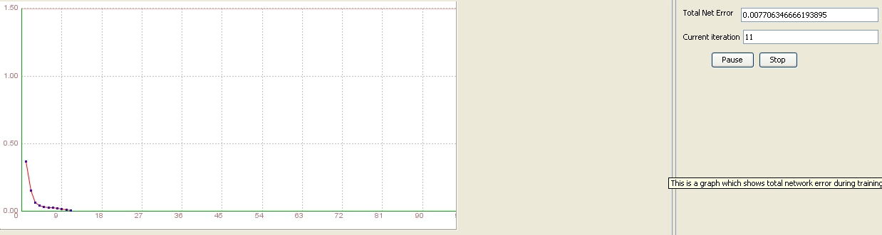
After 11 iterations the network was trained! It succeeded to find the total error beyond the 0.01, more correctly 0.00771, that is less then we had before. But, let's see what the test results will show. Step 6.2 Test the neural network
Now we want to see testing results. 
And Total Mean Square Error is much better that in the previous testing too – about 50% lower, like we wanted. Our statement was correct. Training attempt 3
Step 5.3 Train the neural network
But, let's see what happens if we decrease the Learning rate to 0.1 and the Momentum will remain the same. 
As it was expected, the network need more iterations to find the solution, and more iterations implies more time. After 40 iteration we have total error 0.009882 that is bigger then in earlier attempts. Step 6.3 Test the neural network

The test results are not representative, but with the smaller Learning rate it was expected. Training attempt 4
Even though the previous architecture gave really good results, we will try to lower the number of neurons in hidden layer in order to see what the performances of network will be like then. We are going to use 4 hidden neurons. All other parameters will be the same as before. Step 4.4 Creating a neural network

This is how are architecture look like 
Step 5.4 Train the neural network
The learning parameters will be default values in order to compare these results with the previous one. 
Step 6.4 Test the neural network
Now, we are going to test the network 
The outcome was more then expected! With lower number of hidden neurons then before, the network gave better results. With the same number of iteration, that is 13, the Total Mean Square Error is smaller, 0.00398! Individual error are pretty good too! The final part of testing this network is testing it with several input values. We will select 5 random input values from our data set. Those are:
The output neural network produced for this input is, respectively:
The network guesses all! So far, we can conclude that this is the best solution for our dataset. Let's see what will happen if we put Learnig rate on 0.4 Training attempt 5
Step 5.5 Train the neural network
As we noticed before, if we increase the learning rate, the result will be better. How we are going to see if that is the case with this example too. 
How let's look at the results 
Step 6.5 Test the neural network

We can see that result are better, but not significantly much then in attempt before. It was needed 10 iteration to reach the total mean square error of 0.0036316… that is only 0.00035 lower then previous attempt. We can say that the attempt 5 gave the best results for now. Training attempt 6
Step 4.6 Creating a neural network
We create a new neural network with 2 hidden neurons on one layer. 
The learning parameters will be the same as before in order to compare results. Now train the network and see the results Step 5.6 Train the neural network

Network was successfully trained, now we will test it. Step 6.6 Test the neural network

Results are slightly worse then in 4 hidden architecture. It was needed 24 iteration for training the network, but it succeeded in finding the required error. Total Mean Square Error is also inferior, but not so bad and the individual errors are fine too. But, if we continue to lower down the number of hidden neurons, and put only one hidden neuron and leave default Learning parameters, the network will be not able to do the training successfully. And if the network wasn't successfully trained, therefore is not possible to do testing. So, order to achieve good solution, it is recommended to use more then one and less then five hidden neurons. Until now 4 of them gave the best solution to our problem. Training attempt 7
Step 4.7 Creating a neural network
In this attempt, we will create a different type of neural network. We want to see what will happens if we create neural network with two hidden layers. First we create a new neural network, type will be Multy Layer Perceptron as it was in the previous attempts. Then we put the values 3(space) 2. This means that in first layer we will have 3 hidden neurons, and in second one 2 hidden neurons. 
New neural network has been created, and in the image below is shown the structure of this network. 
Step 5.7 Train the neural network
Now, we are going to train the network and see if it going to give better results then architecture with one hidden layer. The default value of learning parameters will not be changed. 
Step 6.7 Test the neural network

The two layers gave the Network that was successfully trained, therefore the testing was done. We can see that it needed two iteration more then in our best solution, attempt 5, and the Total Mean Square Error is worse then in mentioned case. We can conclude that two hidden layers architecture is able to find the solution, but is not necessary for our problem and we can get better results using just one layer. Advanced training techniques
One of the major advantages of neural networks is their ability to generalize. This means that a trained network can classify data from the same class as the learning data that it has never seen before. This is really big benefit due to the fact in real world applications developers only have a small part of all possible patterns for the generation of a neural network. To do this, we have to divide our training set to two sets- one amount of data will remain training set, and the second one will become the test data. Now, the test set provides a completely independent measure of network accuracy. It is important to emphasize that these two data sets do not have same data. We will try to see how fast and good will network learn if we lower the training set and examine the ability of a network to classify input patterns that are not in the training set. One of the major advantages of neural networks is their ability to generalize. This means that a trained network could classify data from the same class as the learning data that it has never seen before. In real world applications developers normally have only a small part of all possible patterns for the generation of a neural network. To reach the best generalization, the data set should be split into three parts: validation, training and testing set. In the advanced training we are going to use the architecture given in the attempt number 4, that is 13 inputs, 3 outputs, 4 hidden neurons and all other parameters used before. First, we will take 40% of data for training the network and 60% for testing it. Then the relation will be changed, so we are going to use 30% to train and 70 % to test the network. The percentage of training data will continue with descending to 20% and 80% for testing. At the end, we will try to train network with only 10% of data and 90% of data to test it. Let us see how that will work. Training attempt 8
Step 3.8 Create a training set
In this first attempt we will choose random 40% of instances of training set for training and remain 60% for testing. In the initial training set we have 178 instances. This means that now we have 71 instance in training set, and 107 in test set. The Max Error will remain 0.01, Learning Rate 0.2 and Momentum 0.7 Step 5.8 Train the neural network

If we look at the graph above and compare it with the one we had in attempt 4 we will see that the function came close to wanted value after more iteration. We do not have fast decreasing at the beginning like we had before. But still, even with 40% the network succeeded to reach the wanted error value. And what about test results? Here, we test its ability to make judgments for individuals that are not in the training set. Step 6.8 Test the neural network

The Total Mean Square Error is not below 0.01 as we wanted, but close enough. The individual errors are mainly good, but we have some cases where are pretty high (0.835, 0.754…) Training attempt 9
Step 3.9 Create a training set
How we are going to use 30% of data set or 53 instances for training, and 70% that is 125 instances to test the network. Step 5.9 Train the neural network
This will be the brave attempt. We will try with the default parameters, resisting the desire to increase the Learning Rate. 
The network succeeded. The function needed some time to start to fall down, it was not immediately like we have already use to it, but after 26 iteration the total error was below 0.01. Now we have to test it. Step 6.9 Test the neural network

The Total Mean Square Error is expectedly higher, but still the number 0.02272… is still totally perfect. In order to verify the network, we are going to randomly take 5 instances again:
The output neural network produced for this input is, respectively:
As we can see, the network guessed correct in all five instances. Training attempt 10
Step 3.10 Create a training set
In the attempt 11 we are going to use 20% or 53 instances for training, and 80% or 125 instances to test the network. We will be persistent and still not increase neither the Max Error or Learning Rate or Momentum. Step 5.10 Train the neural network

This time, the network also succeeded in reaching the desirable error level. For that it had to make 50 iteration, that is 100% more then in previous attempt. Also, we can see that around 26 iteration it was close to solution, but the network had problems to go beyond the 0.01. Step 6.10 Test the neural network

As we can see, if the parameters remain the same, the result are 100% worse that before even though we increase the test data and decrease the training set by 10%. The Total Mean Square Error is pretty high, more then 40% then we want it to be. Training attempt 11
Step 3.11 Creating a Training Set
The last attempt, but not the least. Now we are going to try to train the network using only 10%, that is 17 instance! Since this is a small number of instances, in order to make the result and network perform better, we will change the Learning Rate to 0.4, but Momentum will stay the same. Step 5.11 Train the neural network
We are going to train the network, and see what the results will be like. 
Even this small number of instances we succeeded to train our network. It took only 32 iteration to have error below the 0.01. Now only what is left to do is to test the network. Step 6.11 Test the neural network

Even though we were using higher value for the Learning Rate, the test results aren't so good as we wanted. Furthermore, in individuals error we have some that are really high 0.8349, 0.7167… But, knowing that we used only 17 instances to train the network, these results are not shocking at all. Conclusion
During this experiment we have created several different architectures of neural networks. Our goal was to find out the architecture structure that will give the best results and to discover its capability to generalize. What proved out to be crucial to the success of the training, is the selection of an appropriate number of hidden neurons during the creating of a new neural network. One hidden layer with more then one neuron in it was perfectly fine to find the really good solutions. We used 17, 4 and 2 hidden neurons, and the best results have been reached with 4 neurons in one hidden layer. Also, through the various tests we demonstrated the sensitivity of neural networks to high and low values of learning parameters. In the end, we divided original data set into two sets- training and testing in order to examine the ability of generation for the architecture with four hidden neurons. We have seen that the network was able to give very good results for cases that have not been presented before. Final results of our experiment are given in the two tables below. In the first table (Table 1.) are the results obtained using standard training techniques, and in the second table (Table 2.) the results obtained by using advanced training techniques. The best solution is indicated by a green background. Table 1. Standard training techniques
Table 2. Advanced training techniques
Download
See also:
Multi Layer Perceptron Tutorial
|

