|
BALANCE SCALE CLASSIFICATION USING NEURAL NETWORKS An example of a multivariate data type classification problem using Neuroph framework by Aleksandra Vojinović, Faculty of Organizational Sciences, University of Belgrade an experiment for Intelligent Systems course Introduction
In this experiment it will be shown how neural networks and Neuroph Studio are used when it comes to problems of classification (assigning data cases to one of a fixed number of possible classes). In classification, the objective is to determine to which of a number of discrete classes a given input case belongs.
Introduction to the problem
We will use Neuroph framework for training the neural network that uses Balance Scale data set.
Balance Scale data set was generated to model psychological experimental results. Each example is classified as having the balance scale tip to the right, tip to the left, or be balanced.The attributes are the left weight, the left distance, the right weight, and the right distance. The correct way to find the class is the greater of (left-distance * left-weight) and (right-distance * right-weight). If they are equal, it is balanced. Main goal of this experiment is to train neural network to classify this 3 type of balance scale. Attribute Information:
Procedure of training a neural network
In order to train a neural network, there are six steps to be made:
In this experiment we will demonstrate the use of some standard and advanced training techniques. Several architectures will be tried out, based on which we will be able to determine what brings us the best results for our problem. Step 1. Data Normalization
In order to train neural network this data set have to be normalized. Normalization implies that all values from the data set should take values in the range from 0 to 1. For that purpose it would be used the following formula: 
Where: X – value that should be normalizedXn – normalized value Xmin – minimum value of X Xmax – maximum value of X Last 3 digits of data set represent class. 1 0 0 represent left class, 0 1 0 balanced class, and 0 0 1 right class. Step 2. Creating a new Neuroph project
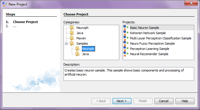
We create a new project in Neuroph Studio by clicking File > New Project, then we choose Neuroph project and click 'Next' button. In a new window we define project name and location. After that we click 'Finish' and a new project is created and will appear in projects window, on the left side of Neuroph Studio. 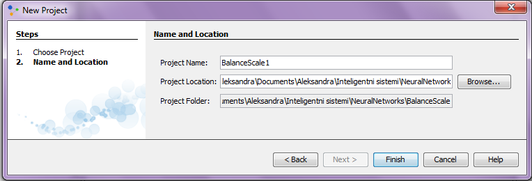 Step 3. Creating a Training Set
To create training set, in main menu we choose Training > New Training Set to open training set wizard. Then we enter name of training set and number of inputs and outputs. In this case it will be 4 inputs and 3 outputs and we will set type of training to be supervised as the most common way of neural network training.
As supervised training proceeds, the neural network is taken through a number of iterations, until the output of the neural network matches the anticipated output, with a reasonably small rate of the error. 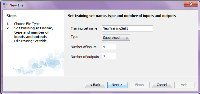
After clicking 'Next' we need to insert data into training set table. All data could be inserted manually, but we have a large number of data instances and it would be a lot more easier to load all data directly from some file. We click on 'Choose File' and select file in which we saved our normalized data set. Values in that file are separated by tab. 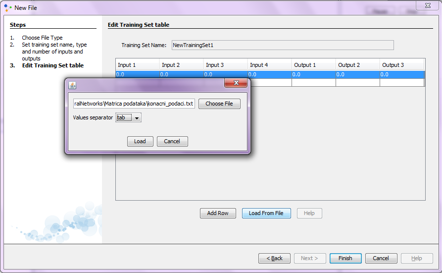
Then, we click 'Load' and all data will be loaded into table. We can see that this table has 7 columns, first 4 of them represents inputs, and last 3 of them represents outputs from our data set. 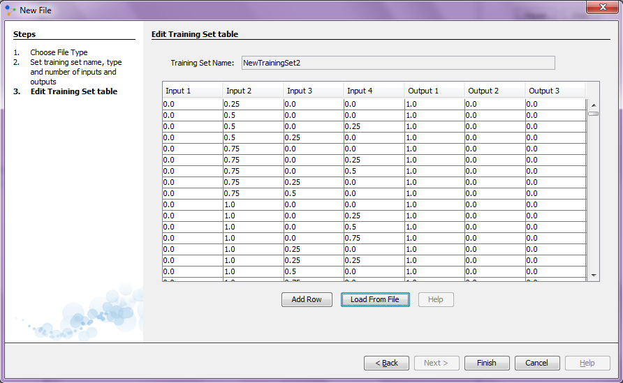
After clicking 'Finish' new training set will appear in our project. Standard training techniques
Standard approaches to validation of neural networks are mostly based on empirical evaluation through simulation and/or experimental testing. There are several methods for supervised training of neural networks. The backpropagation algorithm is the most commonly used training method for artificial neural networks. Backpropagation is a supervised learning method. It requires a data set of the desired output for many inputs, making up the training set. It is most useful for feed-forward networks (networks that have no feedback, or simply, that have no connections that loop). Main idea is to distribute the error function across the hidden layers, corresponding to their effect on the output. Training attempt 1
Step 4.1 Creating a neural network
We create a new neural network by clicking right click on project and then New > Neural Network. Then we define neural network name and type. We will choose 'Multy Layer Perceptron' type. A multilayer perceptron is a feedforward artificial neural network model that maps sets of input data onto a set of appropriate output. It consists of multiple layers of nodes in a directed graph, with each layer fully connected to the next one. Except for the input nodes, each node is a neuron with nonlinear activation function Multylauer perceptron utilizes a supervised learning technique called backpropagation for training the network. It is a modification of the standard linear perceptron, which can distinguish data that is not linearly separable. 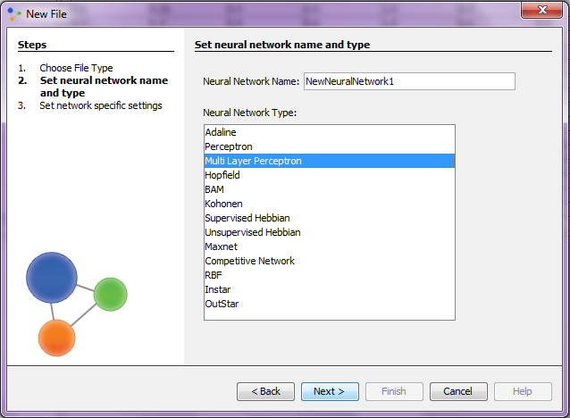
In the next window we will set multy layer perceptron's parameters. The number of input and output neurons are the same as in the training set. And now we have to choose number of hidden layers, and number of neurons in each layer. Problems that require more than one hidden layers are rarely encountered. For many practical problems, there is no reason to use any more than one hidden layer. One layer can approximate any function that contains a continuous mapping from one finite space to another. Deciding the number of hidden neuron layers is only a small part of the problem. We must also determine how many neurons will be in each of these hidden layers. Both the number of hidden layers and the number of neurons in each of these hidden layers must be carefully considered. Using too few neurons in the hidden layers will result in something called underfitting. Underfitting occurs when there are too few neurons in the hidden layers to adequately detect the signals in a complicated data set. Using too many neurons in the hidden layers can result in several problems. First, too many neurons in the hidden layers may result in overfitting. Overfitting occurs when the neural network has so much information processing capacity that the limited amount of information contained in the training set is not enough to train all of the neurons in the hidden layers. A second problem can occur even when the training data is sufficient. An inordinately large number of neurons in the hidden layers can increase the time it takes to train the network. The amount of training time can increase to the point that it is impossible to adequately train the neural network. Obviously, some compromise must be reached between too many and too few neurons in the hidden layers. We’ve decided to have 1 layer and 3 neuron in this first training attempt. Than we check 'Use Bias Neurons' option and choose 'Sigmond' for transfer function (because our data set is normalized). For learning rule we choose 'Backpropagation with Momentum'. The momentum is added to speed up the process of learning and to improve the efficiency of the algorithm. Bias neuron is very important, and the error-back propagation neural network without Bias neuron for hidden layer does not learn. The Bias weights control shapes, orientation and steepness of all types of Sigmoidal functions through data mapping space. A bias input always has the value of 1. Without a bias, if all inputs are 0, the only output ever possible will be a zero. 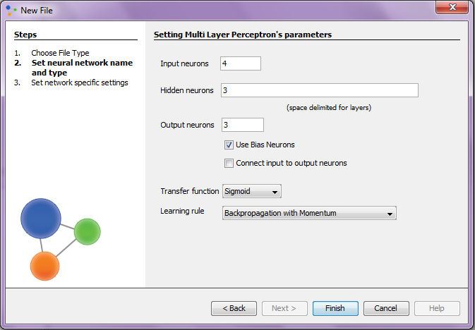
Next, we click 'Finish' and the first neural network is created. In the picture below we can see the graph view of this neural network. 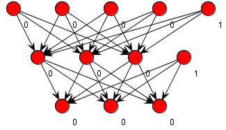 Figure shows the input, the output and hidden neurons and how they are connected with each other. Except for two neurons with activation level 1 (bias activation), all other neurons have an activation level 0. These two neurons represent bias neurons, as we explained above. Step 5.1 Train the neural network
After we have created training set and neural network we can train neural network. First, we select training set, click 'Train', and then we have to set learning parameters for training. Learning rate is a control parameter of training algorithms, which controls the step size when weights are iteratively adjusted. To help avoid settling into a local minimum, a momentum rate allows the network to potentially skip through local minima. A momentum rate set at the maximum of 1.0 may result in training which is highly unstable and thus may not achieve even a local minima, or the network may take an inordinate amount of training time. If set at a low of 0.0, momentum is not considered and the network is more likely to settle into a local minimum. When the Total Net Error value drops below the max error, the training is complete. If the error is smaller we get a better approximation. In this first case a maximum error will be 0.04, learning rate 0.2 and momentum 0.7. 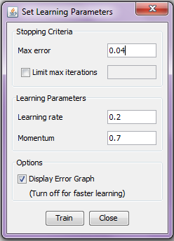
Then we click on the 'Next' button and the training process starts. 
After 45 iterations Total Net Error drop down to a specified level of 0.04 which means that training process was successful and that now we can test this neural network. Step 6.1 Test the neural network
We test neural network by clicking on the 'Test' button, and then we can see testing results. In the results we can see that the Total Mean Square Error is 0.20056347764795712. That certainly is not a very good result, because our goal is to get the total error to be as small as possible. 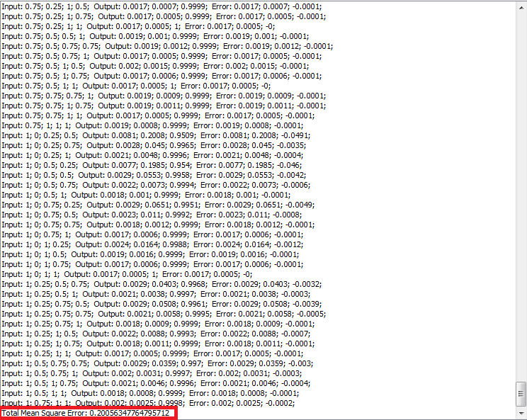
Looking at the individual errors we can observe that most of them are at the low level, below 0.1, but there are also some cases where those errors are considerably larger. So we can conclude that this type of neural network architecture is not the best choice and we should try some other so we could managed to reach the best solution for our problem. Training attempt 2
Step 5.2 Train the neural network
In our second attempt we will only change some learning parameters and then will see what happens. We will decrease the value of a maximum error to 0.03, learning rate will be 0.5 and momentum 0.4. After only 1 iteration it was reached the max error. 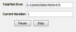
Step 6.2 Test the neural network
Now we want to see testing results. 
In this attempt the total mean square error is even higher then it was in previous case. We should try some other architecture in order to get better results. Training attempt 3
Step 4.3 Creating a neural network
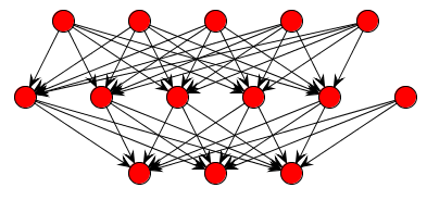
In this attempt we will try to get some better results by increasing the size of hidden neurons. It is known that number of hidden neurons is crucial for network training success, and now we will try with 5 hidden neurons. First we have to create a new neural network. All the parameters are the same as they were in the first training attempt, we will just change the number of hidden neurons. 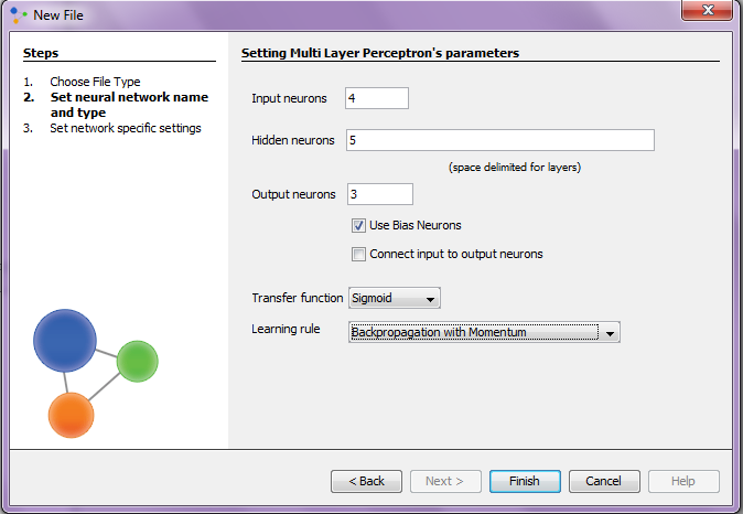
 Step 5.3 Train the neural network
In our first training of this second neural network architecture we will try with the following learning parameters. 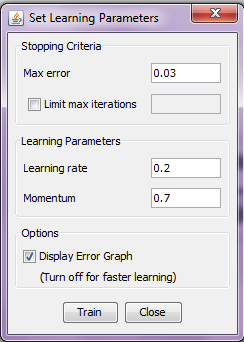 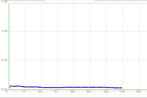
Training process starts, and after 118 iterations it was reached the max error that was given. Step 6.3 Test the neural network
Now, we will test this neural network and see testing results for this neural network architecture. 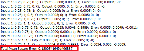 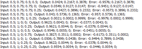
In this case the total mean square error is slightly lower than it was in the last training attempt, but generally the overall result is still not so good. Also, we can see that there are lot of the individual errors that are very high so we will have to try some other network architecture that will give as a better testing results. Training attempt 4
Step 4.4 Creating a neural network
This solution will try to give us a better results than the previous one, with using 7 hidden neurons. All other parameters will be the same as in the previous solutions. 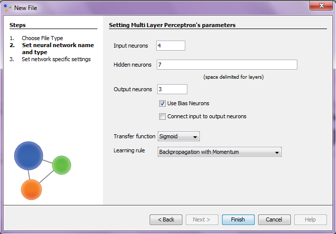
Step 5.4 Train the neural network
Neural network that we've created can now be tested. In this first testing attempt we will set learning parameters as in the picture that is above. 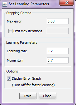 It took 251 iterations for network to train.  Step 6.4 Test the neural network After testing the neural network, we see that the total mean square error is 0.13571201279419912 which is better than it was in the previous attempts, but yet we think that it should be much lower. And also there are still a lot of the individual errors that are near 1 which is pretty bad.  
Training attempt 5
Step 5.5 Train the neural network
In this attempt we will use the same network architecture as it was in the previous training attempt. We will try to get better results by changing some learning parameters. For learning rate now we will set 0.5, and momentum will be 0.4, the max error will remain the same (0.03). 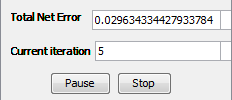
Step 6.5 Test the neural network
After testing, we got that in this attempt the total error is even higher than it was in previous case. 
So we can conclude that 7 neurons isn't enough, and that we should try to use even more hidden neurons. We can only hope that it would bring us to some better results... Training attempt 6
Step 4.6 Creating a neural network
We create a new neural network with 10 hidden neurons on one layer. 
On the image below it is shown the structure of this new neural network. 
Step 5.6 Train the neural network
In this neural network architecture we have 10 hidden neurons, which is even bigger than the sum of inputs and outputs. We think that it should be enough for network to, for the first time, reach the maximum error of 0.01. Learning rate will be 0.2 and momentum 0.7. In this case we will limit the max error to 0.01. Then we will try to train network, and see what happens. 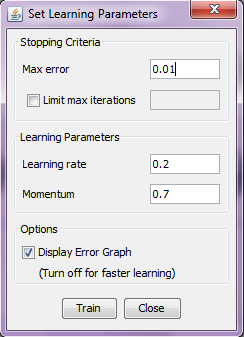
Network was successfully trained, and finally, after 1823 iterations, it was reached a desired error - under 0.01! In the total network error graph we can see that the error decreases continuously throughout the whole training cycle. 
Step 6.6 Test the neural network
We are very interested to see the testing results for this type of neural network architecture. In the training process, the total network error was below 0.01, and that could also indicate a better testing results! After we have finish testing we can see that the total mean square error in this case is 0.07205018979433327, and that certainly is a better than the errors in previous attempts. There are still certain number of high individual errors for some instances, but we can also see that this number represents only about 0.07% of the total number of instances. 
Training attempt 7
Step 5.7 Train the neural network
With this training attempt we will try to reduce the total error by changing some of the learning parameters. Limitation for the max error will remain 0.01, we will increase the learning rate to 0.7 and momentum will be 0.4. As we can see in the image below, network was successfully trained, and after 183 iterations the total error was reduced to the level below 0.01. 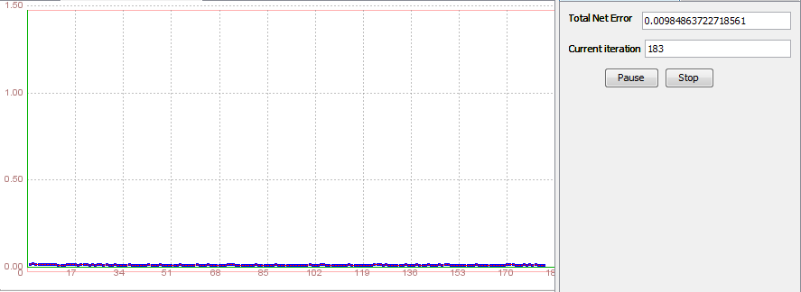
Step 6.7 Test the neural network
After testing neural network, we see that in this attempt the total mean square error is 0.0581858296320496, which is better than the error that was in the previous attempt. But, we still are going to try to find out if it is possible to get even better testing result, with lower total error for the same neural network architecture. 
Training attempt 8
Step 5.8 Train the neural network
In this training attempt we want to see what will happen if we set some even more higher value for learning rate, and lower for momentum. We will set learning rate to be 0.9, and momentum 0.3 and then we will start with neural network training. Training process was successful and after 191 iterations it was reached the total error of 0.01. 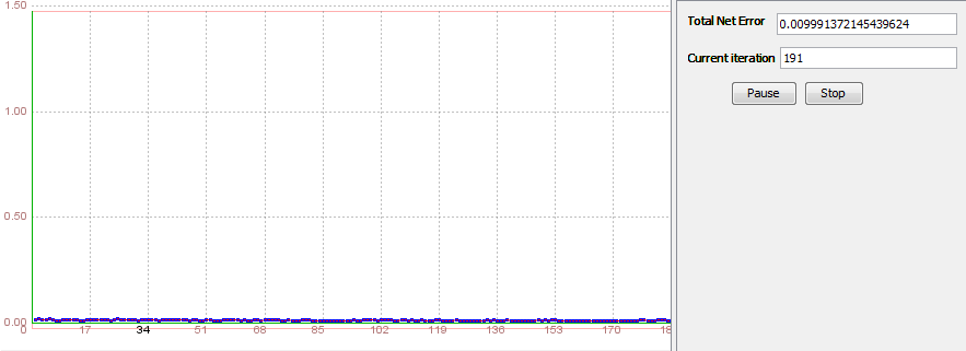
Step 6.8 Test the neural network
After we've done testing, the total mean square error dropped down to the level below 0.03, which is for now the best result that we got for some neural network architecture. 
But anyway, we will try once more to do the training to see if it is possible to get even better results. Training attempt 9
Step 5.9 Train the neural network
Now we want to see how the training process act's if the learning rate and momentum have the same value. In this attempt learning rate and momentum will be 0.4, and maximum error limitation will remain 0.01. We click on the 'Train' button, the training process starts and after 490 iterations it completes successfully. 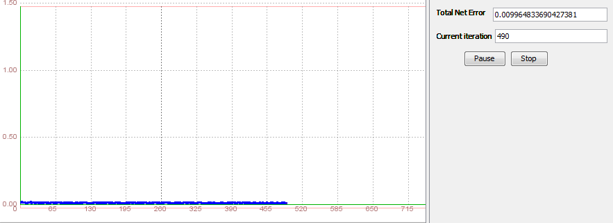
Step 6.9 Test the neural network
We click 'Test' and then we can see testing results for this type of neural network architecture. So far, in this case we've got the best result! For the first time, the total mean square error was under 0.02. 
We also need to examine all the individual errors to make sure that testing was completely successful. We have a large data set so individual testing can require a lot of time. But at the first sight it is obvious that in this case the individual errors are also much smaller than in previous attempts. There are very few extreme cases. For the first time, we will random choose 5 observations which will be subjected to individual testing. Those observations and their testing results are in the following table:
As we can see in the table, the network guessed right in all five cases, so we can conclude that this type of neural network architecture is very good. Training attempt 10
Step 4.10 Creating a neural network
In this attempt, we will create a different type of neural network. We want to see what will happens if we create neural network with two hidden layers. First we create a new neural network, type will be Multy Layer Perceptron as it was in the previous attempts. 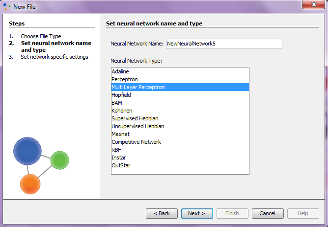
Now we have to set network parameters. We will set 8 neurons on the first layer, and 5 on the second. Learning rule will be Backpropagation with Momentum. 
New neural network has been created, and in the image below is shown the structure of this network. 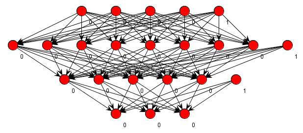
Step 5.10 Train the neural network
Now we will try to train this neural network. First, we have to set training parameters. We will limit the maximum error to 0.01 because we think that this number of neurons in two hidden layers should be enough for network to reach that error. Next we click on 'Train', and the training process starts. Initially, the error was consistently decreased, but after 100 iterations it starts to grow. We let the process continue, but it soon became clear that it is unlikely that the error will fall to below 0.01. Finally, after 23863 iterations we had to stop the training process. 
Network wasn't successfully trained, therefore is not possible to do testing. We can only conclude that more than one hidden layer is not necessary for our problem, and that we can get better results using just one layer. Advanced training techniques
Neural networks represent a class of systems that do not fit into the current paradigms of software development and certification. Instead of being programmed, a learning algorithm “teaches” a neural network using a set of data. Often, because of the non-deterministic result of the adaptation, the neural network is considered a “black box” and its response may not be predictable. Testing the neural network with similar data as that used in the training set is one of the few methods used to verify that the network has adequately learned the input domain. In most instances, such traditional testing techniques prove adequate for the acceptance of a neural network system. However, in more complex, safety- and mission-critical systems, the standard neural network training-testing approach is not able to provide a reliable method for their certification. One of the major advantages of neural networks is their ability to generalize. This means that a trained network could classify data from the same class as the learning data that it has never seen before. In real world applications developers normally have only a small part of all possible patterns for the generation of a neural network. To reach the best generalization, the data set should be split into three parts: validation, training and testing set. The validation set contains a smaller percentage of instances from the initial data set, and is used to determine whether the selected network architecture is good enough. If validation was successful, only then we can do the training. The training set is applied to the neural network for learning and adaptation. The testing set is then used to determine the performance of the neural network by computation of an error metric. This validating-training-testing approach is the first, and often the only, option system developers consider for the assessment of a neural network. The assessment is accomplished by the repeated application of neural network training data, followed by an application of neural network testing data to determine whether the neural network is acceptable. Training attempt 11
Step 3.11 Creating a Training Set
The idea of this attempt is to use only a part of the data set when training a network, and then test the network with inputs from the other, unused part of the data set. That way we can determine whether the neural network has the power of generalization. In the initial training set we have 625 instances. In this attempt we will create a new training set that contains only 20% of initial data set instances and we will pick those instances randomly. First we have to create a new file that would contains new data set instances. A new data set would have 125 instances (11 balanced, 57 left, 57 right). Then, in Neuroph studio we create a new training set, with the same parameters that we used in the first one, and load data from a new data set. We will also create a training set that contains the rest 80% of instances that we should use for network testing later in this attempt. This training set will contains 507 instances (38 balanced, 231 left, 231 right). The final results of this training attempt are shown in Table 2. Step 5.11 Train the neural network
Unlike previous attempts, now we will train some neural network which is already created, but in this case it would be trained with a new created training set which contains 20% instances of the initial training set. For this training we will use neural network which has 10 hidden neurons. Learning rate will be 0.2 and momentum 0.7 in this case. We click on 'Train' button and wait for training process to finish. 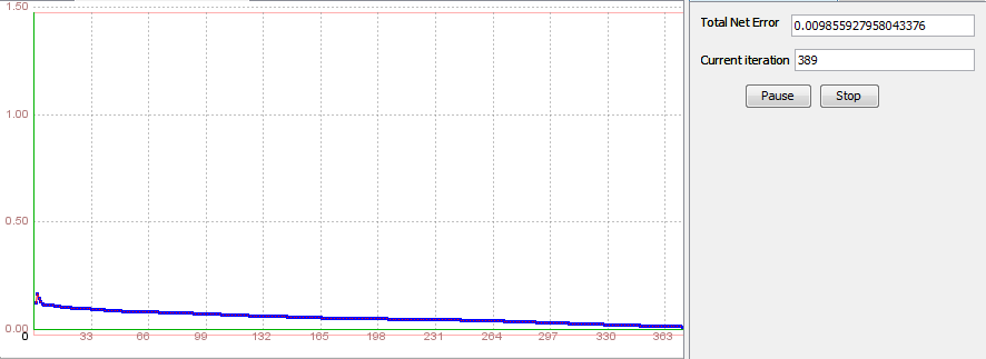
As we can see in the image above, network was successfully trained. It took 389 iterations for training process to finish. Step 6.11 Test the neural network
After successfully training, we can now test neural network. First, will test network with training set that contains only 20% of the initial training set instances. We got that in this case the total error is 0.010110691178851083, which is so far the best result that we got. 
But, the idea was to test neural network with the other 80% of data set that wasn't used for training this neural network. So now, we will try to do that kind of test. This time, for testing, we will use training set that contains the remaining 80% instances that weren't used for training. When training process has completed, we can see that the total error is 0.0550436165797879, which is not so bad considering the fact that we have tested the network with data that was not used during the training. 
Now, we will analyze individual errors by selecting some random inputs to see whether the network is in all cases well predicted the output. We will random choose 5 observations which will be subjected to individual testing. Those observations and their testing results are in the following table:
As we can see in the table, in all 5 times network correctly guessed the output even though the total mean square error was slightly higher. This isn't certainly the best training attempt, but it showed us that this type of network has a good ability of generalization. Training attempt 12
Step 3.12 Creating a Training Set
In this training attempt we will create three different data sets from the initial data set. The first data set will be used for the validation of neural network, the second for training and third for testing the network.
The final results of this training attempt are shown in Table 2. Step 4.12 Creating a neural network
Now, we will create a new neural network. In this attempt we will again try with two hidden layers. On the first layer network will have 3 neurons, and on the second 5 neurons. 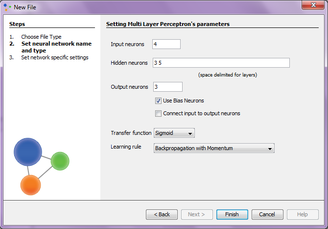
Step 5.12 Validate and Train the neural network
First we need to do a validation of the network by using a smaller set of data so we can check whether such a network architecture is suitable for our problem, and if so, then we can train the network with a larger data set. We will train the network with validation data set that contains 20% of observations. We will set maximum error to be 0.02, learning rate 0.2 and momentum 0.7. Then we click on 'Train' and training starts. Process ends after 369 iterations. 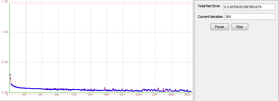
Based on validation, we can conclude that this type of neural network architecture is appropriate, but it is also necessary to train the network with a larger set of data so we can be sure. We will again train this network, but this time with training set that contains 60% of instances. Learning parameters will remain the same as they were during the validation. Unfortunately, it appears that in this case the maximum error of 0.02 was too high, and 40000 iterations were not enough to reach that level of error. We have to stop training. This could mean that in this case we choose a network architecture that does not have enough hidden neurons. 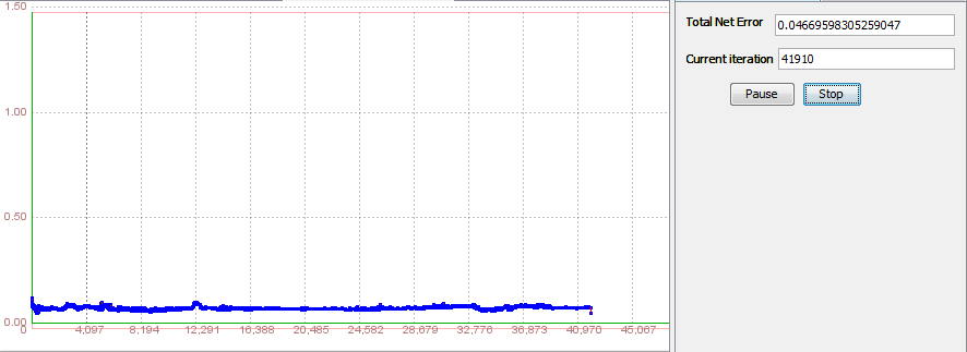
Therefore, after the training has been shown that this type of network architecture is not good enough, so it is not possible to test the network. Training attempt 13
Step 3.13 Creating a training set
In this training attempt we will again create three different data sets from the initial data set: validation, training and testing set.
The final results of this training attempt are shown in Table 2. Step 4.13 Creating a neural network
We will create a new neural network with two hidden layers, first will have 8 neurons, and second will have 4 neurons. 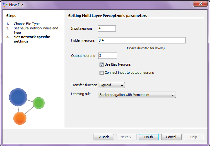
Step 5.13 Validate and Train the neural network
First we need to do a validation of the network by using a smaller set of data so we can check whether such a network architecture is suitable for our problem, and if so, then we can train the network with a larger data set. In this attempt, we will train the network with validation set that uses 25% of observations. Maximum error will be 0.01, learning rate 0.2 and momentum 0.7. Validation was successful, and maximum error was reached after 210 iterations. 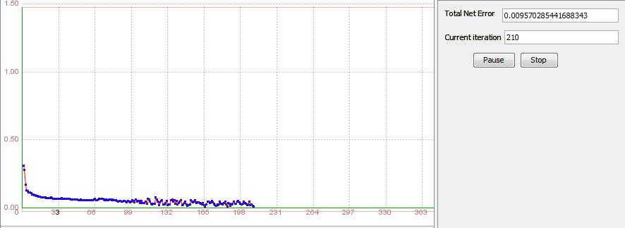
Now, we will train this network with training set that contains 50% of instances. Learning parameters will remain the same. After 233 iterations, the training process was completed successfully. 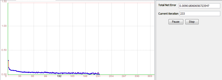
Step 6.13 Test the neural network
Finally, we will test the neural network with testing data set that contains 40% of instances that weren't used during the training and validation. As a result of testing the network, we get a total error of 0.020090939895011466. This is a better result than what we got in the previous attempt in which we've also used the advanced network training techniques. Now if we look at the individual errors, we can see that they are mostly very small which is great. 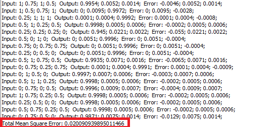
Training attempt 14
Step 3.14 Creating a training set
In this training attempt we will also show the use of advanced training techniques. Three training sets will be created - validation, training, and testing set.
The final results of this training attempt are shown in Table 2. Step 4.14 Creating a neural network
We will create a neural network with two hidden layers, the first will have 9 neurons, and the second 5 neurons. All other parameters will be like in the previous attempt. 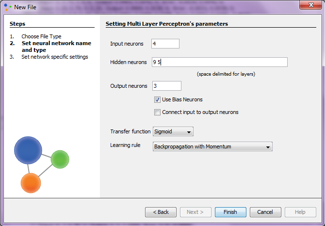
Step 5.14 Validate and Train the neural network
First we need to do a validation of the network by using a smaller set of data so we can check whether such a network architecture is suitable for our problem, and if so, then we can train the network with a larger data set. We will train neural network with validation data set that contains 30% of instances. The maximum error will be 0.01, learning rate 0.4 and momentum 0.6. Training process ends after 105 instances. 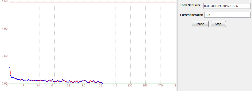
Then we need to train the neural network with training set that contains 70% of instances using the same learning parameters. After 1290 iterations process ends, and we can see that training was successful. 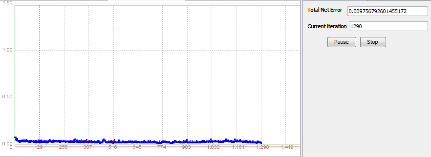
Step 6.14 Test the neural network
Now we need to test this neural network in order to see results. The total mean square error in this case is slightly larger than in the previous attempt, and is 0.029320642171416958. So, we can conclude that although in this attempt we increased the number of neurons in both layers, it did not bring us a better result than the result from the previous attempt. 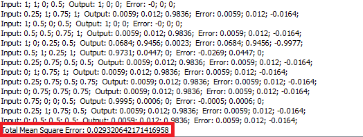
Conclusion
During this experiment, we have created several different architectures of neural networks. We wanted to find out what is the most important thing to do during the neural network training in order to get the best results. What proved out to be crucial to the success of the training, is the selection of an appropriate number of hidden neurons during the creating of a new neural network. One hidden layer is in most cases proved to be sufficient for the training success. As it turned, in our experiment was better to use more neurons. We have tried by using 3, 5 and 7 hidden neurons, but we've got the best results by using 10 neurons. Also, through the various tests we have demonstrated the sensitivity of neural networks to high and low values of learning parameters. We have shown the difference between standard and advanced training techniques. Final results of our experiment are given in the two tables below. In the first table (Table 1.) are the results obtained using standard training techniques, and in the second table (Table 2.) the results obtained by using advanced training techniques. The best solution is indicated by a green background. Table 1. Standard training techniques
Table 2. Advanced training techniques
Download
See also:
Multi Layer Perceptron Tutorial
| |||||||||||||||||||||||||||||||||||||||||||||||||||||||||||||||||||||||||||||||||||||||||||||||||||||||||||||||||||||||||||||||||||||||||||||||||||||||||||||||||||||||||||||||||||||||||||||||||||||||||||||||||||||||||||||||||||||||||||||||||||||||||||||||||||||||||||||||||||||||||||||||||||||||||||||||||||||||||||||||||||||||||||||||||||||||||||||||||||||||||||||||||||||||||||||||||||


