
|
GLASS IDENTIFICATION USING NEURAL NETWORKS An example of a multivariate data type classification problem using Neuroph framework by Ivana Čutović, Faculty of Organizational Sciences, University of Belgrade an experiment for Intelligent Systems course Introduction
The term neural network was traditionally used to refer to a network or circuit of biological neurons. The modern usage of the term often refers to artificial neural networks, which are composed of artificial neurons or nodes. Neural networks, as used in artificial intelligence, have traditionally been viewed as simplified models of neural processing in the brain, even though the relation between this model and brain biological architecture is debated, as it is not clear to what degree artificial neural networks mirror brain function. In more practical terms neural networks are non-linear statistical data modeling or decision making tools. They can be used to model complex relationships between inputs and outputs or to find patterns in data. However, the paradigm of neural networks - i.e., implicit, not explicit , learning is stressed - seems more to correspond to some kind of natural intelligence than to the traditional symbol-based Artificial Intelligence, which would stress, instead, rule-based learning.
Neural networks have seen an explosion of interest over the last few years, because they are being successfully applied across an extraordinary range of problem domains, in areas as diverse as finance, medicine, engineering, geology and physics. Indeed, anywhere that there are problems of prediction, classification or control, neural networks are being introduced. Neural networks learn by example. The neural network user gathers representative data, and then invokes training algorithms to automatically learn the structure of the data. Although the user does need to have some heuristic knowledge of how to select and prepare data, how to select an appropriate neural network, and how to interpret the results, the level of user knowledge needed to successfully apply neural networks is much lower than would be the case using some more traditional nonlinear statistical methods.
In this experiment it will be shown how neural networks and Neuroph Studio are used when it comes to problems of classification (assigning data cases to one of a fixed number of possible classes). In classification, the objective is to determine to which of a number of discrete classes a given input case belongs.
Introduction to the problem
We will use Neuroph framework for training the neural network that uses Glass Identification data set.
Glass Identification data set was generated to help in criminological investigation. At the scene of the crime, the glass left
can be used as evidence, but only if it is correctly identified. Each example is classified as building_windows_float_processed, building_windows_non_float_processed, vehicle_windows_float_processed, vehicle_windows_non_float_processed (none in this database), containers, tableware and headlamps.The attributes are RI: refractive index, Na: Sodium (unit measurement: weight percent in corresponding oxide, as are attributes 4-10), Mg: Magnesium, Al: Aluminum, Si: Silicon, K: Potassium, Ca: Calcium, Ba: Barium, Fe: Iron. Main goal of this experiment is to train neural network to classify this 7 types of glass. Attribute Information:
Procedure of training a neural network
In order to train a neural network, there are six steps to be made:
In this experiment we will demonstrate the use of some standard and advanced training techniques. Several architectures will be tried out, based on which we will be able to determine what brings us the best results for our problem. Step 1. Data Normalization
In order to train neural network this data set have to be normalized. Normalization implies that all values from the data set should take values in the range from 0 to 1. For that purpose it would be used the following formula: 
Where: X – value that should be normalizedXn – normalized value Xmin – minimum value of X Xmax – maximum value of X Last 7 digits of data set represent class: 1 0 0 0 0 0 0 represent building_windows_float_processed 0 1 0 0 0 0 0 building_windows_non_float_processed class 0 0 1 0 0 0 0 vehicle_windows_float_processed class 0 0 0 1 0 0 0 vehicle_windows_non_float_processed (none in this database) 0 0 0 0 1 0 0 containers class 0 0 0 0 0 1 0 tableware class 0 0 0 0 0 0 1 headlamps class Step 2. Creating a new Neuroph project
We create a new project in Neuroph Studio by clicking File > New Project, then we choose Neuroph project and click 'Next' button. In a new window we define project name and location. After that we click 'Finish' and a new project is created and will appear in projects window, on the left side of Neuroph Studio. 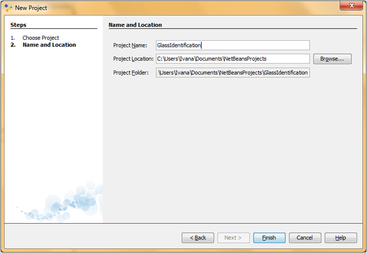 Step 3. Creating a Training Set
To create training set, in main menu we choose Training > New Training Set to open training set wizard. Then we enter name of training set and number of inputs and outputs. In this case it will be 9 inputs and 7 outputs and we will set type of training to be supervised as the most common way of neural network training.
As supervised training proceeds, the neural network is taken through a number of iterations, until the output of the neural network matches the anticipated output, with a reasonably small rate of the error. 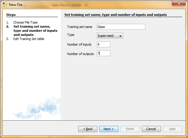
After clicking 'Next' we need to insert data into training set table. All data could be inserted manually, but we have a large number of data instances and it would be a lot more easier to load all data directly from some file. We click on 'Choose File' and select file in which we saved our normalized data set. Values in that file are separated by tab.   Then, we click 'Load' and all data will be loaded into table, and after clicking 'Finish' new training set will appear in our project.  To be able to decide which is the best solution for our problem we will create several neural networks, with different sets of parameters, and most of them will be based on this training set. Standard training techniques
Standard approaches to validation of neural networks are mostly based on empirical evaluation through simulation and/or experimental testing. There are several methods for supervised training of neural networks. The backpropagation algorithm is the most commonly used training method for artificial neural networks. Backpropagation is a supervised learning method. It requires a data set of the desired output for many inputs, making up the training set. It is most useful for feed-forward networks (networks that have no feedback, or simply, that have no connections that loop). Main idea is to distribute the error function across the hidden layers, corresponding to their effect on the output. Training attempt 1
Step 4.1 Creating a neural network
We create a new neural network by clicking right click on project and then New > Neural Network. Then we define neural network name and type. We will choose 'Multy Layer Perceptron' type. A multilayer perceptron is a feedforward artificial neural network model that maps sets of input data onto a set of appropriate output. It consists of multiple layers of nodes in a directed graph, with each layer fully connected to the next one. Except for the input nodes, each node is a neuron with nonlinear activation function Multylauer perceptron utilizes a supervised learning technique called backpropagation for training the network. It is a modification of the standard linear perceptron, which can distinguish data that is not linearly separable. 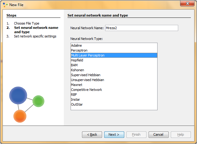
Now we will set multy layer perceptron's parameters. The number of input and output neurons are the same as in the training set (so 9 inputs and 7 outputs). And than we have to choose number of hidden layers, and number of neurons in each layer. Problems that require more than one hidden layers are rarely encountered. For many practical problems, there is no reason to use any more than one hidden layer. One layer can approximate any function that contains a continuous mapping from one finite space to another.The decision about number of hidden neurons isn't the only problem in training networks. We must also determine how many neurons will be in each of these hidden layers. Both the number of hidden layers and the number of neurons in each of these hidden layers must be carefully considered. Using too few neurons in the hidden layers will result in something called underfitting. Underfitting occurs when there are too few neurons in the hidden layers to adequately detect the signals in a complicated data set. Using too many neurons in the hidden layers can result in several problems. First, too many neurons in the hidden layers may result in overfitting. Overfitting occurs when the neural network has so much information processing capacity that the limited amount of information contained in the training set is not enough to train all of the neurons in the hidden layers. A second problem can occur even when the training data is sufficient. An inordinately large number of neurons in the hidden layers can increase the time it takes to train the network. The amount of training time can increase to the point that it is impossible to adequately train the neural network. Obviously, some compromise must be reached between too many and too few neurons in the hidden layers. We’ve decided to have 1 layer and 2 neuron in this first training attempt. Than we check 'Use Bias Neurons' option and choose 'Sigmond' for transfer function (because our data set is normalized). For learning rule we choose 'Backpropagation with Momentum'. The momentum is added to speed up the process of learning and to improve the efficiency of the algorithm. Bias neuron is very important, and the error-back propagation neural network without Bias neuron for hidden layer does not learn. The Bias weights control shapes, orientation and steepness of all types of Sigmoidal functions through data mapping space. A bias input always has the value of 1. Without a bias, if all inputs are 0, the only output ever possible will be a zero. 
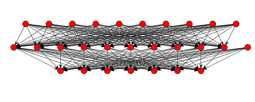
Next, we click 'Finish' and the first neural network is created. In the picture below we can see the graph view of this neural network. 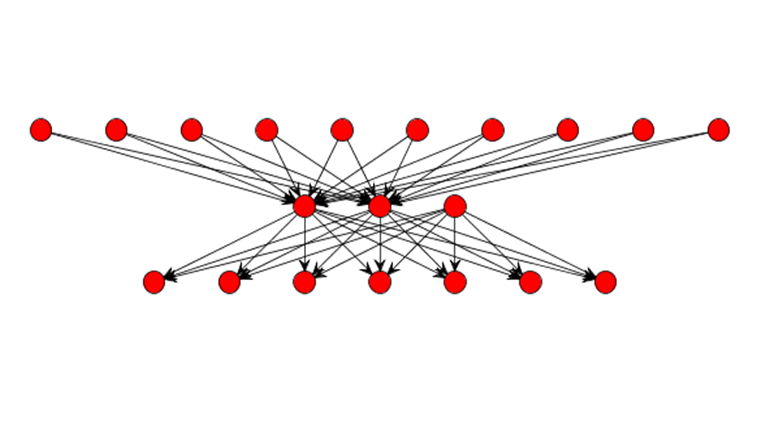 Figure shows the input, the output and hidden neurons and how they are connected with each other. Except for two neurons with activation level 1 (bias activation), all other neurons have an activation level 0. These two neurons represent bias neurons, as we explained above. Step 5.1 Train the neural network
After we have created training set and neural network we can train neural network. First, we select training set, click 'Train', and then we have to set learning parameters for training. Learning rate is a control parameter of training algorithms, which controls the step size when weights are iteratively adjusted. To help avoid settling into a local minimum, a momentum rate allows the network to potentially skip through local minima. A momentum rate set at the maximum of 1.0 may result in training which is highly unstable and thus may not achieve even a local minima, or the network may take an inordinate amount of training time. If set at a low of 0.0, momentum is not considered and the network is more likely to settle into a local minimum. When the Total Net Error value drops below the max error, the training is complete. If the error is smaller we get a better approximation. In this first case a maximum error will be 0.04, learning rate 0.2 and momentum 0.7. 
Then we click on the 'Train' button and the training process starts. 
 Network fails to converge after reasonable period and training is not complete after 73806 iterations. Training is not completed so we can’t test the network. Training attempt 2
Step 5.2 Train the neural network
In our second attempt let us try to change some learning parameters and then will see what happens. In network window click Randomize button and then click Train button. We will leave the same value of a maximum error, learning rate will be 0.3 and momentum 0.5. After very large number of iteration max error wasn't reached.  In the table below for the next three sessions we will present the results of other trainings for the first architecture. For other trainings is not given graphic. Table 1 Training results for the first architecture
Training attempt 7
Step 4.7 Creating a neural network
In this attempt we will try to get some better results by increasing the size of hidden neurons. It is known that number of hidden neurons is crucial for network training success, and now we will try with 10 hidden neurons. First we have to create a new neural network. All the parameters are the same as they were in the first training attempt, we will just change the number of hidden neurons. 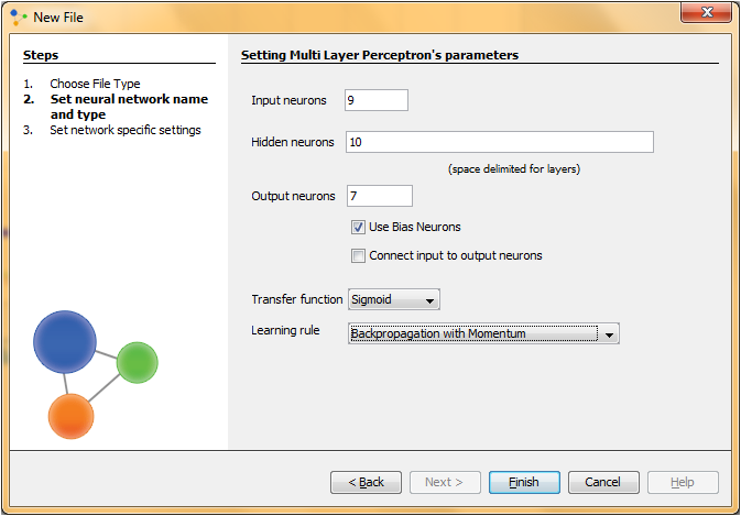
 Step 5.7 Train the neural network
In training of this second neural network architecture we will try with the following learning parameters. In the table below we can see all combination of learning parameters that we used, and the errors that we achieved. Number of iterations is limited on 5000, because the rasults for training werent significant even after 60 000 iterations, so we have shown these training just for example. Table 2 Training results for 10 hidden neurons architecture
Now, we see that we need another network architecture to find apropriate solution. Training attempt 10
Step 4.10 Creating a neural network
This solution will try to give us a better results than the previous one, with using 20 hidden neurons and the same training set.First training course, of third architecture, we will start with default values of learning rate and momentum. First click on button Train. In Set Learning parameters dialog,fill in field set Stopping criteria with value 0.01 as max error. We wont limit number of iterations this time After entering this values click on button Train. Step 5.10 Train the neural network
Neural network that we've trained had shown growing error tendency so we intreupted training.During the testing we unsuccessfully trained the neural network named Mreza20.   Training attempt 11
Step 5.11 Train the neural network
In this attempt we will use the same network architecture as it was in the previous training attempt. We will try to get better results by changing some learning parameters. We will try out twice bigger learning rate, and smaller momentum value. For learning rate now we will set the value 0.4, and momentum will be 0.5, the max error will be 0.03. 
As we can see, changing the learning parameters decreesed the total net error, but it didn't got us 0.03 max error, so we will try out some more similar changes for lerning parameters. The summary of the results are shown in the Table 3. Table 3 Training results for 20 hidden neurons architecture
So we can conclude that 20 neurons isn't enough, and that we should try to use even more hidden neurons. Training attempt 14
Step 4.14 Creating a neural network
Because we havent succeeded to decerease total net error in previous atempts, we will create a new neural network with even more hidden neurons on one layer. After we tried out 10 and 20 hidden neurons, we will now create new network with 30 hidden neurons. We 'll do it the same way as in previous atempts. Step 5.14 Train the neural network
In this neural network architecture we have 30 hidden neurons, which is even bigger than the sum of inputs and outputs. We think that it should be enough for network to, for the first time, reach the maximum error of 0.01. Learning rate will be 0.2 and momentum 0.7, as it already set as default. In this case we will limit the max error to 0.01. Then we will try to train network, and see what happens. 
From the graphics can be seen from iteration to iteration there are no large shifts in the prediction. More accurate in predicting, fluctuations are very small and the values are around 0.2. So we are moving to our next combination of hidden neurons and learning parameters. Training attempt 15
Step 4.15 Creating a neural network
We create a new neural network with 40 hidden neurons on one layer which is even twice bigger than the sum of input and output neurons. This drastic solution is chosen because we concluded that our previous trainings had no or small shifts in prediction. That's why we hope that this much complex neural network may give us apropriate clasification for our data set. Step 5.15 Train the neural network
Now we will train this new network. We will use as parameters 0.1 for learning rate, 0.4 for momentum, max error will reamin as default 0.01. 
Network was successfully trained, and finally, after 29417 iterations, it was reached a desired error - under 0.01! In the total network error graph we can see that the error decreases continuously throughout the whole training cycle. Step 6.15 Test the neural network
As we already mentioned above, we could not test the network after training the previous architecture, because the total error is not reached a satisfactory level. Now we are now able to test network to make sure that it is trained properly. Go to network window and click button Test, and then we can see testing results for this type of neural network architecture. So far, in this case we've got the best result! 
Training attempt 16
We also want to see if there were solutions with less than 29417 iterations. In our next training we will set bigger momentum, 0.5, and the other two parameters will remain the same. 

The other attempts with this network and comparison of theit total net errors will be shown in table below. Table 4.1 Training results for 40 hidden neurons architecture
We also need to examine all the individual errors to make sure that testing was completely successful. We have a large data set so individual testing can require a lot of time. But at the first sight it is obvious that in this case the individual errors are also much smaller than in previous attempts. There are very few extreme cases. For the first time, we will random choose 5 observations which will be subjected to individual testing. Those observations and their testing results are in the following table: Table 4.2 Values of inputs
Table 4.3 Values of outputs
As with other statistical methods, and classification using neural networks include errors that arise during the approximation. Individual error between the original and the assessed values are shown in Table 3.3. Table 4.4 Individual errors
As we can see in all three tables, the network guessed right in all five cases, so we can conclude that this type of neural network architecture is very good. Advanced training techniques
Neural networks represent a class of systems that do not fit into the current paradigms of software development and certification. Instead of being programmed, a learning algorithm “teaches” a neural network using a set of data. Often, because of the non-deterministic result of the adaptation, the neural network is considered a “black box” and its response may not be predictable. Testing the neural network with similar data as that used in the training set is one of the few methods used to verify that the network has adequately learned the input domain. In most instances, such traditional testing techniques prove adequate for the acceptance of a neural network system. However, in more complex, safety- and mission-critical systems, the standard neural network training-testing approach is not able to provide a reliable method for their certification. One form of regularization is to split the training set into a new training set and a validation set. After each step through the new training set, the neural network is evaluated on the validation set. The network with the best performance on the validation set is then used for actual testing. Your new training set consisted of the say it for example 70% - 80% of the original training set, and the remaining 30% - 20% would be classified in the validation set. Then you have to compute the validation error rate periodically during training and stop training when the validation error rate starts to go up. However, validation error is not a good estimate of the generalization error, if your initial set consists of a relatively small number of instances. Our initial set, we named it dataSetGlass, consists only of 214 instances . In this case 20% or 30%, of the original training set, consisted of small amount of instances. This is the insufficient number of instances to perform validation. In this case instead validation we will use a generalization as a form of regularization. One way to get appropriate estimate of the generalization error is to run the neural network on the test set of data that is not used at all during the training process. The generalization error is usually defined as the expected value of the square of the difference between the learned function and the exact target. In the following examples we will check the generalization error, such as from the example to the example we will increase the number of instances in the training set, which we use for training, and we will decrease the number of instances in the sets that we used for testing. Training attempt 19
Step 3.19 Creating a Training Set
The idea of this attempt is to use only a part of the data set when training a network, and then test the network with inputs from the other, unused part of the data set. That way we can determine whether the neural network has the power of generalization. In the initial training set we have 214 instances. In this attempt we will create a new training set that contains only 30% randomly chosen data of initial data set instances. First we have to create a new file that would contains new data set instances. A new data set would have 64 instances (9 instances of group 7, 3 from group 6, 4 from group 5, none of group 4, 5 from group 3, 22 from group 2 and 21 from group 1). Then, in Neuroph studio we create a new training set named 20%data, with the same parameters that we used in the first one, and load data from a new data set. We will also create a training set that contains the rest 70% of instances that we should use for network testing later in this attempt. This training set will contains 150 instances . Step 5.19 Train the neural network
Unlike previous attempts, now we will train some neural network which is already created, but in this case it would be trained with a new created training set which contains 70% instances of the initial training set. For this training we will use neural network which has 10 hidden neurons. Learning rate will be 0.1 and momentum 0.5 in this case. We click on 'Train' button and wait for training process to finish. 
As we can see in the image above, network was successfully trained. It took 362 iterations for training process to finish. Step 6.19 Test the neural network
After successful training we should test the data. The idea was to test neural network with the other 30% of data set that wasn't used for training this neural network. So now, we will try to do that kind of test. This time, for testing, we will use training set that contains the remaining 30% instances that weren't used for training. Summary of theese trainings are given in the table below. 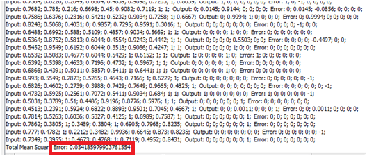
Table 5 Advance training results for given architecture
Conclusion
During this experiment, we have created several different architectures of neural networks. We wanted to find out what is the most important thing to do during the neural network training in order to get the best results. We tried to understand the behavior of theese neural netvorks through trying different parametres and different amount of data. We can only agree that crucial thig that brings the success of the training, is selecting the most suitable number of hidden neurons during creating a new neural network. One hidden layer is in most cases proved to be sufficient for the training success. As it turned, in our experiment was better to use more neurons. We have tried by using 2, 10, 20, 30 and 40 hidden neurons, but we've got the best results by using 40 neurons. Also, through the various tests we have demonstrated the sensitivity of neural networks to high and low values of learning parameters. We have shown the difference between standard and advanced training techniques. Final results of our experiment are given in table below. In this table are the results obtained using standard and advanced training techniques. Table 6 Standard and advanced training techniques
Download
Data set used in this tutorial
See also:
Multi Layer Perceptron Tutorial
| |||||||||||||||||||||||||||||||||||||||||||||||||||||||||||||||||||||||||||||||||||||||||||||||||||||||||||||||||||||||||||||||||||||||||||||||||||||||||||||||||||||||||||||||||||||||||||||||||||||||||||||||||||||||||||||||||||||||||||||||||||||||||||||||||||||||||||||||||||||||||||||||||||||||||||||||||||||||||||||||||||||||||||||||||||||||||||||||||||||||||||||||||||||||||||||||||||||||||||||||||||||||||||||||||||||||||||||||||||||||||||||||||||||||||||||||||||||||||||||||||||||||||||||||||||||||||||||||||||||||||||||||||||||||||||||||||||||||||||


