
|
LENSES CLASSIFICATION USING NEURAL NETWORKS An example of a multivariate data type classification problem using Neuroph framework by Maja Urosevic, Faculty of Organizational Sciences, University of Belgrade an experiment for Intelligent Systems course Introduction
An Artificial Neural Network (ANN) is an information processing paradigm that is inspired by the way biological nervous systems,
such as the brain, process information. The key element of this paradigm is the novel structure of the information processing system. It is composed of a large number of
highly interconnected processing elements (neurones) working in unison to solve specific problems. ANNs, like people, learn by example. Neural networks,
with their remarkable ability to derive meaning from complicated or imprecise data, can be used to extract patterns and detect trends that are too complex
to be noticed by either humans or other computer techniques. A trained neural network can be thought of as an "expert" in the category of information
it has been given to analyse. This expert can then be used to provide projections given new situations of interest and answer "what if" questions. Other advantages include:
Introduction to the problem
Neuroph framework will be used to train the neural network that uses Database for fitting contact lenses (Lenses data set). The dataset used is taken from a paper
by Cendrowska (1988) on the inductive analysis of a set of ophthalmic data. The lenses data set tries to predict whether a person will need soft contact lenses,
hard contact lenses or no contacts, by determining relevant attributes of the client.The data set has 4 attributes (age of the patient, spectacle prescription, notion on astigmatism, and information on tear production rate) plus an associated three-valued class, that gives the appropriate lens prescription for patient (hard contact lenses, soft contact lenses, no lenses). The data set contains 24 instances(class distribution: hard contact lenses- 4, soft contact lenses-5, no contact lenses- 15).
Attribute Information: (the first attribute of the data set is an ID number, and therefore, has not been included in the training set)
Procedure of training a neural network
In order to train a neural network, there are six steps to be made:
Several architectures have been tried out during the experiment in order to find the best solution to the given problem. Step 1. Transform the data set
Since attributes in this data set are categorical, we have to express them in digits, which means we will look at every attribute as if it were a class an instance belongs to.
Let us consider, for example, the attribute Age of the patient, which has 3 possible values. If the observed instance has value 1 for the attribute (represents a young person),
we will put 1 0 0 for the values of this attribute and so on.
The last 3 digits of the data set represent the class an instance belongs to. 1 0 0 represent hard contact lenses class, 0 1 0 soft contact lenses class, and 0 0 1 no contact lenses class. The original data set can be dowloaded here. The transformed data set can be downloaded here. Step 2. Creating a new Neuroph project
We create a new project in Neuroph Studio by clicking File > New Project, next we choose Neuroph project and click 'Next' button.
Next step is to define project name and location. After that, we click 'Finish' and the created project will appear in Projects window. 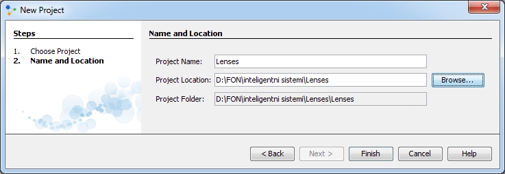 Step 3. Creating a Training Set
To create a training set, in the main menu we have to choose Training > New Training Set. Then we enter a name for our training set as well as numbers of inputs and outputs,
which, in this case, are 9 and 3. The type of training is set to supervised as the most common way of neural network training.
During the training, neural network is taken through a number of iterations, until the output of the neural network matches the anticipated output, with a reasonably low error rate. 
After clicking 'Next', we should insert our data set into training set table. We will load all data directly from a file, by clicking on 'Choose File' and selecting the one where we saved our transformed data set. Values in the file are separated by tab. 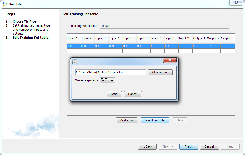
By clicking on 'Load', all our data will be loaded into a table. We can see that this table has 12 columns, where the first 9 of them represent inputs, and the last 3 represent outputs from our data set. 
After clicking 'Finish' a new training set will appear in our project. Training techniques
Standard approaches to validation of neural networks are mostly based on empirical evaluation through simulation and/or experimental testing. There are several methods for supervised training of neural networks. The backpropagation algorithm is the most commonly used training method for artificial neural networks. Backpropagation is a common method of training artificial neural networks so as to minimize the objective function. It requires a data set of the desired output for many inputs, making up the training set. It is most useful for feed-forward networks (networks that have no feedback, or simply, that have no connections that loop). Main idea is to distribute the error function across the hidden layers, corresponding to their effect on the output. Training attempt 1
Step 4.1 Creating a neural network
We create a new neural network by right clicking on project and then New > Neural Network.
Next we define our neural network name and type, which will be 'Multi Layer Perceptron' in our case. A multilayer perceptron is a feedforward artificial neural network model that maps sets of input data onto a set of appropriate output. It consists of multiple layers of nodes in a directed graph, with each layer fully connected to the next one. Except for the input nodes, each node is a neuron with a nonlinear activation function. Multilayer perceptron utilizes backpropagation for training the network. It is a modification of the standard linear perceptron, which can distinguish data that is not linearly separable. 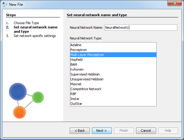
In the next window we set parameters of the network. Numbers of input and output neurons are the same as in the training set. We decide the number of hidden layers as well as the number of neurons in each layer. Problems that require more than one hidden layer are rarely encountered. For many practical problems, there is no reason to use more than one hidden layer. One layer can approximate any function that contains a continuous mapping from one finite space to another. Deciding about the number of hidden neuron layers is only a small part of the problem. We must also determine how many neurons in each of the hidden layers will be. Both the number of hidden layers and the number of neurons in each of these hidden layers must be carefully considered. Using too few neurons in the hidden layers will result in something called underfitting. Underfitting occurs when there are too few neurons in the hidden layers to adequately detect the signals in a complicated data set. Using too many neurons in the hidden layers can result in several problems. Firstly, too many neurons in the hidden layers may result in overfitting. Overfitting occurs when the neural network has so much information processing capacity that the limited amount of information contained in the training set is not enough to train all of the neurons in the hidden layers. A second problem can occur even when the training data is sufficient. An inordinately large number of neurons in the hidden layers can increase the time it takes to train the network. The amount of training time can increase to the point that it is impossible to adequately train the neural network. Obviously, some compromise must be reached between too many and too few neurons in the hidden layers. We have chosen 1 layer with 8 hidden neurons in this first training attempt. We check 'Use Bias Neurons' option and choose 'Sigmoid' for transfer function in all our networks. For learning rule we choose 'Backpropagation with Momentum'. The momentum is added to speed up the process of learning and to improve the efficiency of the algorithm. Bias neuron is very important, and the error-back propagation neural network without Bias neuron for hidden layer does not learn. Neural networks are "unpredictable" to a certain extent so if you add a bias neuron you're more likely to find solutions faster then if you didn't use a bias. The Bias weights control shapes, orientation and steepness of all types of Sigmoidal functions through data mapping space. A bias input always has the value of 1. Without a bias, if all inputs are 0, the only output ever possible will be a zero. 
Next, we click 'Finish' and the first neural network is created. In the picture below we can see the graph view of this neural network.  The graph shows the input, output, hidden neurons and how they are connected with each other. Except for the two neurons with activation level 1 (bias activation), all other neurons have an activation level 0. These two neurons represent bias neurons, as we explained above. Step 5.1 Train the neural network
After we have created the training set and the neural network, we can train it. Firstly, we select our training set, click 'Train', and then set learning parameters for the training. Learning rate is a control parameter of training algorithms, which controls the step size when weights are iteratively adjusted. To help avoid settling into a local minimum, a momentum rate allows the network to potentially skip through local minimum. A momentum rate set at the maximum of 1.0 may result in training which is highly unstable and thus may not achieve even a local minimum, or the network may take an inordinate amount of training time. If set at a low of 0.0, momentum is not considered and the network is more likely to settle into a local minimum. When the Total Net Error value drops below the max error, the training is complete. The smaller the error, the better the approximation. In this case, we set the maximum error to 0.01, learning rate to 0.2 and momentum to 0.7. 
Then we click on the 'Next' button and the training process starts. 
After 49 iterations Total Net Error drops down to a specified level of 0.01 which means that training process was successful and that now we can test this neural network. Step 6.1 Test the neural network
We test the neural network by clicking on the 'Test' button. In the results we can see that the Total Mean Square Error is 0.00516061449608549. That is certainly a very good result, because our goal is to get the total error smaller than 0,01. 
Looking over the individual errors we realize that all of them are at the low level, below 0.01. It means that this neural network architecture is acceptable. Still, we will try to find better results by changing learning parameters. Training attempt 2
Step 5.2 Train the neural network
In our second attempt we will only change the learning rate and see what happens. We will set it to 0.6. Momentum stays the same as before. After only 22 iterations, the max error was reached. 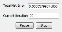
Step 6.2 Test the neural network
Now we look at the testing results. 
In this attempt the total mean square error is lower than in the previous case. We will now look for different architectures to find out if we can get even better results than this one. Training attempt 3
Step 4.3 Creating a neural network
In this attempt we will try to get better results by reducing the number of hidden neurons to 5. It is known that the number of hidden neurons is crucial for the success of network training. At first we create a new neural network. All the parameters are the same as they were in the first training attempt, we only change the number of hidden neurons. 
 Step 5.3 Train the neural network
We will train the network with the following learning parameters:  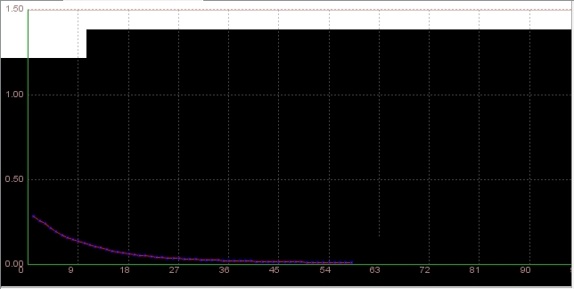
It took 58 iterations to reach the max error of 0,01. 
Step 6.3 Test the neural network
Now, we will test this neural network and see testing results for this neural network architecture. 
In this case the total mean square error is slightly higher than it was in the last training attempt, but generally the overall result is good. We will try to find even better result with a lower number of hidden neurons. Training attempt 4
Step 4.4 Creating a new neural network
In this attempt, we will try to achieve a better result by using 4 hidden neurons. 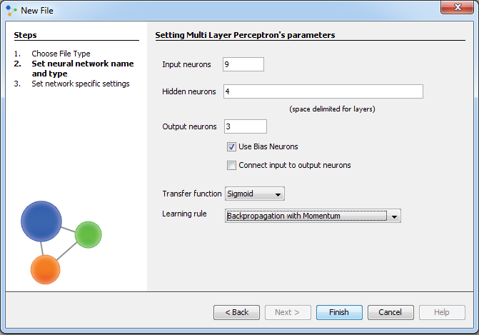
Step 5.4 Train the neural network
The neural network we have created can now be trained. In the first testing attempt we will set learning parameters as in the picture below:  It took 55 iterations for network to train.  Step 6.4 Test the neural network After testing the neural network, we see that the total mean square error is 0.005698442819583745. It is very similar to the results from previous attempts, but yet we think that it could be lower. 
Training attempt 5
Step 5.5 Train the neural network
In this attempt we will use the same network architecture as it was in the previous training attempt. We will try to get even better results by changing some learning parameters. We will put 0.6 for the learning rate and 0.7 for momentum, while the max error will stay the same. 
Step 6.5 Test the neural network
After testing, we got that in this attempt the total error is lower than it was in previous case with learning rate 0.2. 
So we can conclude that 4 neurons are enough, but we will still try to find an architecture with a lower number of neurons that will give us the best result. Training attempt 6
Step 5.6 Train the neural network
In this attempt we will use the same network architecture as it was in the previous training attempt. We will try to get even better results by changing some learning parameters. We will put 0.4 for the learning rate and 0.5 for momentum, while max error will stay the same. 
Step 6.6 Test the neural network
After testing, the total error is lower than it was in the case with learning rate 0.2, but higher than in the case with learning rate 0.6 and momentum 0.7. 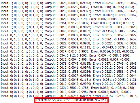
The conclusion is that with 4 hidden neurons, the best result is achieved when putting the learning rate higher than 0.2. Also, we should not decrease momentum too much in order to get a low total error. Training attempt 7
Step 4.7 Creating a neural network
We will create a new neural network with 3 hidden neurons. 
Step 5.7 Train the neural network
In this neural network architecture we have 3 hidden neurons. We will see if that is enough for the network to reach the maximum error of 0.01. For the beginning, learning rate will be 0.2 and momentum 0.7. 
Network was successfully trained, and after 64 iterations, the desired error was reached. In the total network error graph we can see that the error decreases continuously throughout the whole training cycle. 
Step 6.7 Test the neural network
After we have finished testing, we can see that the total mean square error in this case is slightly higher than the errors in previous attempts, so we will try to improve that by changing learning parameters and see what happens. 
Training attempt 8
Step 5.8 Train the neural network
With this training attempt we will try to reduce the total error by changing some of the learning parameters. Limitation for the max error will remain 0.01, we will increase the learning rate to 0.4 and decrease momentum- it will be 0.4. As we can see in the image below, network was successfully trained, and after 73 iterations the total error was reduced to the level below 0.01. 
Step 6.8 Test the neural network
After testing the neural network, we see that in this attempt the total mean square error is 0.0056955553861498635, which is better than the error that was in the previous attempt . But, we are still going to try to find out if it is possible to get even better testing result, with lower total error for the same neural network architecture. 
Training attempt 9
Step 5.9 Train the neural network
In this training attempt we want to see what will happen if we set higher values for both the learning rate and momentum. We will put 0.6 for the learning rate and 0.7 for momentum. Training process was successful and after 24 iterations, the total error of 0.01 was reached. 
Step 6.9 Test the neural network
This is the best result achieved with 3 hidden neurons, so the conclusion is to increase the learning rate in this architecture. 
Training attempt 10
Step 4.10 Creating a neural network
We will create a new neural network with 2 hidden neurons. 
Step 5.10 Train the neural network
In this neural network architecture we have 2 hidden neurons. We will see if that is enough for the network to reach the maximum error of 0.01. Firstly, we set learning rate to 0.2 and momentum to 0.7. 
Network was successfully trained, and, after 49 iterations, the desired error was reached. 
Step 6.10 Test the neural network
After we have finished the testing, we see that the total mean square is quite low. Still, we will try to find if there is a combination of learning parameters that will give us the best possible result so far. 
Training attempt 11
Step 5.11 Train the neural network
In this training attempt we want to see what will happen if we set even higher value for the learning rate- 0.7, while the momentum stays the same. Training process was successful and after 53 iterations the desired error was reached. 
Step 6.11 Test the neural network
This was the best result achieved with 2 hidden neurons, and also the best result achieved since the beginning of the experiment! 
Training attempt 12
Step 4.12 Creating a neural network
In this attempt, we will create a different type of neural network. We want to see what will happen if we create a neural network with two hidden layers. We will put 3 neurons in the first layer, and 2 in the second. 
The structure of the new network is shown in the graph below: 
Step 5.12 Train the neural network
We will see if these 2 layers are enough for the network to reach the maximum error of 0.01. We will put 0.2 for the learning rate and 0.7 for momentum. 
Training process was successful and after 119 iterations the desired error was reached. 
Step 6.12 Test the neural network
The result achieved with two hidden layers is also acceptable, since the total mean square error is 0.005599376700513674. 
All in all, there is no need for using more than one hidden layer, since we did not get better results than those from using only one hidden layer. The final results of all training attempts are shown in Table 1. Conclusion
In the experiment, we have trained several architectures of neural networks. The goal was to find out the most important factor in determining the best results. The selection of an appropriate number of hidden neurons during the creating of a new neural network proved to be crucial for our aim. One hidden layer was sufficient for the training success in all cases. We tried out the training of different networks, but we wanted to achieve the lowest error with the lowest number of hidden neurons. We used 8, 5, 4, 3 and 2 hidden neurons and we succeeded in getting the best result with 2 neurons. Also, the experiment showed that the success of a neural network is very sensitive to learning parameters chosen in the training process. The overall conclusion would be that the higher the learning rate, the faster the network is trained. We recommend using a high learning rate and a moderate momentum to optimize the classification performance and the number of iterations. The final results of our experiment using standard training techniques are given in the table below. The best solution is indicated by a grey background. Table 1. Training techniques
Download
See also:
Multi Layer Perceptron Tutorial
|


