|
Car Evaluation Dataset Test
An example of a multivariate data type classification problem using Neuroph
by Tijana Jovanovic, Faculty of Organisation Sciences, University of Belgrade
an experiment for Intelligent Systems course
Introduction
In this example we will be testing Neuroph with Car Dataset, which can be found : here. Several architectures will be tried out, and it will be determined which ones represent a good solution to the problem, and which ones does not.
First here are some useful information about our Car Dataset:
Data Set Characteristics: Multivariate
Number of Instances: 1728
Attribute Characteristics: Categorical
Number of Attributes: 6
Associated Tasks: Classification
Introducing the problem
Car Evaluation Database was derived from a simple hierarchical decision model.
The model evaluates cars according to the following concept structure:
CAR: car acceptability
. . PRICE overall price
. . buying buying price
. . maint price of the maintenance
. . COMFORT comfort
. . doors number of doors
. . persons capacity in terms of persons to carry
. . lug_boot the size of luggage boot
. . safety estimated safety of the car
Six input attributes: buying, maint, doors, persons, lug_boot, safety.
Attribute Information:
Class Values:
unacc, acc, good, vgood
Attributes:
buying: vhigh, high, med, low.
maint: vhigh, high, med, low.
doors: 2, 3, 4, 5more.
persons: 2, 4, more.
lug_boot: small, med, big.
safety: low, med, high.
For this experiment to work we had to transform our data set in binary format (0, 1).We replaced each attribute value with suitable binary combination.
For example,the attribute buying has 4 posible values:vhigh, high, med, low.Since these values are in a String format we had to transform each in a number format.So in this case each string value will be replaced with a combination of 4 binary numbers.The final transformation looks like this:
Attributes:
buying: 1,0,0,0 instead of vhigh, 0,1,0,0 instead of high, 0,0,1,0 instead of med, 0,0,0,1 instead of low.
maint: 1,0,0,0 instead of vhigh, 0,1,0,0 instead of high, 0,0,1,0 instead of med, 0,0,0,1 instead of low.
doors: 0,0,0,1 instead of 2, 0,0,1,0 instead of 3, 0,1,0,0 instead of 4, 1,0,0,0 instead of 5more.
persons: 0,0,1 instead of 2, 0,1,0 instead of 4, 1,0,0 instead of more.
lug_boot: 0,0,1 instead of small, 0,1,0 instead of med, 1,0,0 instead of big.
safety: 0,0,1 instead of low, 0,1,0 instead of med, 1,0,0 instead of high.
Transformed Dataset
In this example we will be using 80% of data for training the network and 20% of data for testing it.
Before you start reading our experiment we suggest to first get more familiar with Neuroph Studio and Multi Layer Perceptron.You can do that by clicking on the links below:
Neuroph Studio Geting started
Multi Layer Perceptron
Training attempt 1
Here you can see the structure of our network with its inputs,outputs and hidden neurons in the middle layer.

Network Type: Multi Layer Perceptron
Training Algorithm: Backpropagation with Momentum
Number of inputs: 21
Number of outputs: 4 (unacc,acc,good,vgood)
Hidden neurons: 14
Training Parameters:
Learning Rate: 0.2
Momentum: 0.7
Max. Error: 0.01
Training Results:
For this training, we used Sigmoid transfer function.

As you can see, the neural network took 33 iterations to train. Total Net Error is acceptable 0.0095
Total Net Error graph look like this:

Practical Testing:

The final part of testing this network is testing it with several input values. To do that, we will select 5 random input values from our data set. Those are:
|
Network Inputs |
Real Outputs |
Instance number |
Buying |
Maint |
Doors |
Persons |
Lug boot |
Safety |
Unacc |
Acc |
Good |
VGood |
| 1. |
0,0,0,1(vhigh) |
0,0,0,1(vhigh) |
1,0,0,0(2) |
1,0,0(2) |
0,1,0,(med) |
0,1,0(med) |
1 |
0 |
0 |
0 |
| 2. |
1,0,0,0 (low) |
1,0,0,0 (low) |
0,0,0,1 (5more) |
0,1,0 (4) |
0,0,1 (big) |
0,0,1 (high) |
0 |
0 |
0 |
1 |
| 3. |
1,0,0,0 (low) |
1,0,0,0 (low) |
0,0,0,1 (5more) |
0,1,0 (4) |
1,0,0 (small) |
1,0,0 (low) |
1 |
0 |
0 |
0 |
| 4. |
1,0,0,0 (low) |
1,0,0,0 (low) |
0,0,0,1 (5more) |
0,0,1 (more) |
1,0,0 (small) |
0,1,0 (med) |
0 |
1 |
0 |
0 |
| 5. |
1,0,0,0 (low) |
0,1,0,0 (med) |
0,0,0,1 (5more) |
0,1,0 (4) |
0,0,1 (big) |
0,1,0 (med) |
0 |
0 |
1 |
0 |
The output neural network produced for this input is, respectively:
|
Network Inputs |
Outputs neural network produced |
Instance number |
Buying |
Maint |
Doors |
Persons |
Lug boot |
Safety |
Unacc |
Acc |
Good |
VGood |
| 1. |
0,0,0,1(vhigh) |
0,0,0,1(vhigh) |
1,0,0,0(2) |
1,0,0(2) |
0,1,0,(med) |
0,1,0(med) |
1 |
0 |
0 |
0 |
| 2. |
1,0,0,0 (low) |
1,0,0,0 (low) |
0,0,0,1 (5more) |
0,1,0 (4) |
0,0,1 (big) |
0,0,1 (high) |
0,0009 |
0,0002 |
0,0053 |
0,9931 |
| 3. |
1,0,0,0 (low) |
1,0,0,0 (low) |
0,0,0,1 (5more) |
0,1,0 (4) |
1,0,0 (small) |
1,0,0 (low) |
1 |
0 |
0,0001 |
0 |
| 4. |
1,0,0,0 (low) |
1,0,0,0 (low) |
0,0,0,1 (5more) |
0,0,1 (more) |
1,0,0 (small) |
0,1,0 (med) |
0,0033 |
0,9965 |
0,0025 |
0 |
| 5. |
1,0,0,0 (low) |
0,1,0,0 (med) |
0,0,0,1 (5more) |
0,1,0 (4) |
0,0,1 (big) |
0,1,0 (med) |
0,0002 |
0,0006 |
0,9973 |
0,0016 |
The network guessed correct in all five instances. After this test, we can conclude that this solution does not need to be rejected. It can be used to give good results in most cases.
In our next experiment we will be using the same network,but some of the parametres will be different and we will see how the result is going to change.
Training attempt 2
Network Type: Multi Layer Perceptron
Training Algorithm: Backpropagation with Momentum
Number of inputs: 21
Number of outputs: 4 (unacc,acc,good,vgood)
Hidden neurons: 14
Training Parameters:
Learning Rate: 0.3
Momentum: 0.6
Max. Error: 0.01
Training Results:
For this training, we used Sigmoid transfer function.

As you can see, the neural network took 21 iterations to train. Total Net Error is acceptable 0.0098
Total Net Error graph look like this:

Practical Testing:

The only thing left is to put the random inputs stated above into the neural network. The result of the test are shown in the table. The network guessed right in all five cases.
|
Network Inputs |
Outputs neural network produced |
Instance number |
Buying |
Maint |
Doors |
Persons |
Lug boot |
Safety |
Unacc |
Acc |
Good |
VGood |
| 1. |
0,0,0,1(vhigh) |
0,0,0,1(vhigh) |
1,0,0,0(2) |
1,0,0(2) |
0,1,0,(med) |
0,1,0(med) |
1 |
0 |
0 |
0 |
| 2. |
1,0,0,0 (low) |
1,0,0,0 (low) |
0,0,0,1 (5more) |
0,1,0 (4) |
0,0,1 (big) |
0,0,1 (high) |
0 |
0 |
0 |
0,9996 |
| 3. |
1,0,0,0 (low) |
1,0,0,0 (low) |
0,0,0,1 (5more) |
0,1,0 (4) |
1,0,0 (small) |
1,0,0 (low) |
1 |
0 |
0 |
0 |
| 4. |
1,0,0,0 (low) |
1,0,0,0 (low) |
0,0,0,1 (5more) |
0,0,1 (more) |
1,0,0 (small) |
0,1,0 (med) |
0 |
1 |
0 |
0 |
| 5. |
1,0,0,0 (low) |
0,1,0,0 (med) |
0,0,0,1 (5more) |
0,1,0 (4) |
0,0,1 (big) |
0,1,0 (med) |
0 |
0 |
1 |
0 |
As we can see from this table,network guessed allmost every instance in this test without any error,so we can say that the second combination of parametres is even better than the first one.
In the next two attempts we will be making a new neural network.The main difference will be the number of hidden neurons in the structure of our network and other parametres will also be changed.
Training attempt 3
Network Type: Multi Layer Perceptron
Training Algorithm: Backpropagation with Momentum
Number of inputs: 21
Number of outputs: 4 (unacc,acc,good,vgood)
Hidden neurons: 10
Training Parameters:
Learning Rate: 0.3
Momentum: 0.6
Max. Error: 0.01
Training Results:
For this training, we used Sigmoid transfer function.

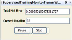
As you can see, the neural network took 37 iterations to train. Total Net Error is acceptable 0.00995
Total Net Error graph look like this:

Practical Testing:

The final part of testing this network is testing it with several input values. To do that, we will select 5 random input values from our data set. Those are:
|
Network Inputs |
Real Outputs |
Instance number |
Buying |
Maint |
Doors |
Persons |
Lug boot |
Safety |
Unacc |
Acc |
Good |
VGood |
| 1. |
0,0,0,1(vhigh) |
0,0,0,1(vhigh) |
1,0,0,0(2) |
1,0,0(2) |
0,1,0,(med) |
0,1,0(med) |
1 |
0 |
0 |
0 |
| 2. |
1,0,0,0 (low) |
1,0,0,0 (low) |
0,0,0,1 (5more) |
0,1,0 (4) |
0,0,1 (big) |
0,0,1 (high) |
0 |
0 |
0 |
1 |
| 3. |
1,0,0,0 (low) |
1,0,0,0 (low) |
0,0,0,1 (5more) |
0,1,0 (4) |
1,0,0 (small) |
1,0,0 (low) |
1 |
0 |
0 |
0 |
| 4. |
1,0,0,0 (low) |
1,0,0,0 (low) |
0,0,0,1 (5more) |
0,0,1 (more) |
1,0,0 (small) |
0,1,0 (med) |
0 |
1 |
0 |
0 |
| 5. |
1,0,0,0 (low) |
0,1,0,0 (med) |
0,0,0,1 (5more) |
0,1,0 (4) |
0,0,1 (big) |
0,1,0 (med) |
0 |
0 |
1 |
0 |
The output neural network produced for this input is, respectively:
|
Network Inputs |
Outputs neural network produced |
Instance number |
Buying |
Maint |
Doors |
Persons |
Lug boot |
Safety |
Unacc |
Acc |
Good |
VGood |
| 1. |
0,0,0,1(vhigh) |
0,0,0,1(vhigh) |
1,0,0,0(2) |
1,0,0(2) |
0,1,0,(med) |
0,1,0(med) |
1 |
0,0001 |
0 |
0 |
| 2. |
1,0,0,0 (low) |
1,0,0,0 (low) |
0,0,0,1 (5more) |
0,1,0 (4) |
0,0,1 (big) |
0,0,1 (high) |
0 |
0,001 |
0,0129 |
0,986 |
| 3. |
1,0,0,0 (low) |
1,0,0,0 (low) |
0,0,0,1 (5more) |
0,1,0 (4) |
1,0,0 (small) |
1,0,0 (low) |
1 |
0 |
0 |
0 |
| 4. |
1,0,0,0 (low) |
1,0,0,0 (low) |
0,0,0,1 (5more) |
0,0,1 (more) |
1,0,0 (small) |
0,1,0 (med) |
0,0033 |
0,9935 |
0,0045 |
0 |
| 5. |
1,0,0,0 (low) |
0,1,0,0 (med) |
0,0,0,1 (5more) |
0,1,0 (4) |
0,0,1 (big) |
0,1,0 (med) |
0 |
0,0191 |
0,9568 |
0,0237 |
The network guessed correct in all five instances. After this test, we can conclude that this solution does not need to be rejected. It can be used to give good results in most cases.
In our next experiment we will be using the same network,but some of the parametres will be diferent and we will see how the result is going to change.
Training attempt 4
Network Type: Multi Layer Perceptron
Training Algorithm: Backpropagation with Momentum
Number of inputs: 21
Number of outputs: 4 (unacc,acc,good,vgood)
Hidden neurons: 10
Training Parameters:
Learning Rate: 0.5
Momentum: 0.7
Max. Error: 0.01
Training Results:
For this training, we used Sigmoid transfer function.

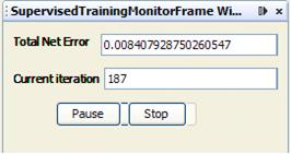
As you can see, the neural network took 187 iterations to train. Total Net Error is acceptable 0.0084
Total Net Error graph look like this:

Practical Testing:

The only thing left is to put the random inputs stated above into the neural network. The result of the test are shown in the table. The network guessed right in all five cases.
|
Network Inputs |
Outputs neural network produced |
Instance number |
Buying |
Maint |
Doors |
Persons |
Lug boot |
Safety |
Unacc |
Acc |
Good |
VGood |
| 1. |
0,0,0,1(vhigh) |
0,0,0,1(vhigh) |
1,0,0,0(2) |
1,0,0(2) |
0,1,0,(med) |
0,1,0(med) |
1 |
0 |
0 |
0 |
| 2. |
1,0,0,0 (low) |
1,0,0,0 (low) |
0,0,0,1 (5more) |
0,1,0 (4) |
0,0,1 (big) |
0,0,1 (high) |
0 |
0 |
0 |
1 |
| 3. |
1,0,0,0 (low) |
1,0,0,0 (low) |
0,0,0,1 (5more) |
0,1,0 (4) |
1,0,0 (small) |
1,0,0 (low) |
1 |
0 |
0 |
0 |
| 4. |
1,0,0,0 (low) |
1,0,0,0 (low) |
0,0,0,1 (5more) |
0,0,1 (more) |
1,0,0 (small) |
0,1,0 (med) |
0 |
1 |
0,0094 |
0 |
| 5. |
1,0,0,0 (low) |
0,1,0,0 (med) |
0,0,0,1 (5more) |
0,1,0 (4) |
0,0,1 (big) |
0,1,0 (med) |
0 |
0,0736 |
0,9996 |
0 |
Training attempt 5
This time we will be making some more significant changes in the structure of our network.Now we will try to train a network with 5 neurons in its hidden layer.
Network Type: Multi Layer Perceptron
Training Algorithm: Backpropagation with Momentum
Number of inputs: 21
Number of outputs: 4 (unacc,acc,good,vgood)
Hidden neurons: 5
Training Parameters:
Learning Rate: 0.2
Momentum: 0.7
Max. Error: 0.01
Training Results:
We stoped the trening of network at this number of iterations because it is obious that in this case the network is not going to be trained succesfully and will not be able to learn the data from the set.
Total Net Error graph look like this:

So the conclusion of this experiment is that the choice of the number of hidden neurons is crucial to the effectiveness of a neural network.
One of the "rules" for determining the correct number of neurons to use in the hidden layers is that the number of hidden neurons should be between the size of the input layer and the size of the output layer.Formula that we used looks like this:((number of inputs + number of outputs)/2)+1.In that case we made a good network that showed great results.Then we made a network with less neurons in its hidden layer and the results were not as good as before.So,in the next example we are going to see how will the network react with a greater number of hidden neurons.
Training attempt 6
Network Type: Multi Layer Perceptron
Training Algorithm: Backpropagation with Momentum
Number of inputs: 21
Number of outputs: 4 (unacc,acc,good,vgood)
Hidden neurons: 17
Training Parameters:
Learning Rate: 0.2
Momentum: 0.7
Max. Error: 0.01
Training Results:
For this training, we used Sigmoid transfer function.

As you can see, the neural network took 23 iterations to train. Total Net Error is acceptable 0.0099
Total Net Error graph look like this:

Practical Testing:

The final part of testing this network is testing it with several input values. To do that, we will select 5 random input values from our data set. Those are:
|
Network Inputs |
Real Outputs |
Instance number |
Buying |
Maint |
Doors |
Persons |
Lug boot |
Safety |
Unacc |
Acc |
Good |
VGood |
| 1. |
0,0,0,1(vhigh) |
0,0,0,1(vhigh) |
1,0,0,0(2) |
1,0,0(2) |
0,1,0,(med) |
0,1,0(med) |
1 |
0 |
0 |
0 |
| 2. |
1,0,0,0 (low) |
1,0,0,0 (low) |
0,0,0,1 (5more) |
0,1,0 (4) |
0,0,1 (big) |
0,0,1 (high) |
0 |
0 |
0 |
1 |
| 3. |
1,0,0,0 (low) |
1,0,0,0 (low) |
0,0,0,1 (5more) |
0,1,0 (4) |
1,0,0 (small) |
1,0,0 (low) |
1 |
0 |
0 |
0 |
| 4. |
1,0,0,0 (low) |
1,0,0,0 (low) |
0,0,0,1 (5more) |
0,0,1 (more) |
1,0,0 (small) |
0,1,0 (med) |
0 |
1 |
0 |
0 |
| 5. |
1,0,0,0 (low) |
0,1,0,0 (med) |
0,0,0,1 (5more) |
0,1,0 (4) |
0,0,1 (big) |
0,1,0 (med) |
0 |
0 |
1 |
0 |
The output neural network produced for this input is, respectively:
|
Network Inputs |
Outputs neural network produced |
Instance number |
Buying |
Maint |
Doors |
Persons |
Lug boot |
Safety |
Unacc |
Acc |
Good |
VGood |
| 1. |
0,0,0,1(vhigh) |
0,0,0,1(vhigh) |
1,0,0,0(2) |
1,0,0(2) |
0,1,0,(med) |
0,1,0(med) |
1 |
0,0001 |
0 |
0 |
| 2. |
1,0,0,0 (low) |
1,0,0,0 (low) |
0,0,0,1 (5more) |
0,1,0 (4) |
0,0,1 (big) |
0,0,1 (high) |
0,0002 |
0,0001 |
0,0073 |
0,9946 |
| 3. |
1,0,0,0 (low) |
1,0,0,0 (low) |
0,0,0,1 (5more) |
0,1,0 (4) |
1,0,0 (small) |
1,0,0 (low) |
0,9987 |
0,0012 |
0,0002 |
0 |
| 4. |
1,0,0,0 (low) |
1,0,0,0 (low) |
0,0,0,1 (5more) |
0,0,1 (more) |
1,0,0 (small) |
0,1,0 (med) |
0,0031 |
0,9912 |
0,0236 |
0 |
| 5. |
1,0,0,0 (low) |
0,1,0,0 (med) |
0,0,0,1 (5more) |
0,1,0 (4) |
0,0,1 (big) |
0,1,0 (med) |
0 |
0,0191 |
0,9568 |
0,0237 |
As you can see,this number of hidden neurons with appropriate combination of parametres also gave a good results and guessed all five instances.
Training attempt 7
Now we will see how the same network is going to work with a diferent set of parametres.
Network Type: Multi Layer Perceptron
Training Algorithm: Backpropagation with Momentum
Number of inputs: 21
Number of outputs: 4 (unacc,acc,good,vgood)
Hidden neurons: 17
Training Parameters:
Learning Rate: 0.6
Momentum: 0.2
Max. Error: 0.02
Training Results:
For this training, we used Sigmoid transfer function.

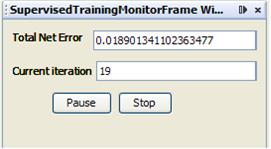
As you can see, the neural network took 19 iterations to train. Total Net Error is acceptable 0.0189
Total Net Error graph look like this:

Practical Testing:

The only thing left is to put the random inputs stated above into the neural network. The result of the test are shown in the table. The network guessed right in all five cases.
|
Network Inputs |
Outputs neural network produced |
Instance number |
Buying |
Maint |
Doors |
Persons |
Lug boot |
Safety |
Unacc |
Acc |
Good |
VGood |
| 1. |
0,0,0,1(vhigh) |
0,0,0,1(vhigh) |
1,0,0,0(2) |
1,0,0(2) |
0,1,0,(med) |
0,1,0(med) |
0,9997 |
0 |
0 |
0 |
| 2. |
1,0,0,0 (low) |
1,0,0,0 (low) |
0,0,0,1 (5more) |
0,1,0 (4) |
0,0,1 (big) |
0,0,1 (high) |
0,0002 |
0,0009 |
0,0232 |
0,9973 |
| 3. |
1,0,0,0 (low) |
1,0,0,0 (low) |
0,0,0,1 (5more) |
0,1,0 (4) |
1,0,0 (small) |
1,0,0 (low) |
1 |
0 |
0 |
0 |
| 4. |
1,0,0,0 (low) |
1,0,0,0 (low) |
0,0,0,1 (5more) |
0,0,1 (more) |
1,0,0 (small) |
0,1,0 (med) |
0,0015 |
0,9952 |
0,0075 |
0 |
| 5. |
1,0,0,0 (low) |
0,1,0,0 (med) |
0,0,0,1 (5more) |
0,1,0 (4) |
0,0,1 (big) |
0,1,0 (med) |
0,0001 |
0,0525 |
0,9886 |
0,0193 |
Although in this example we used considerably different set of parametres the network gave a good results in the test.
Advanced training techniques
This chapter will show another technique for training a neural network that involves validation and generalization.So far we were training the network with the 80% of our data and tested it with the rest (20%).Now we will be trying out different combinations such as : 70%:30% and 60%:40% ans see if we can find any noticable differences beetween them.
Training attempt 8
Now we are using 70% of data for training and 30% for testing the network.
Network Type: Multi Layer Perceptron
Training Algorithm: Backpropagation with Momentum
Number of inputs: 21
Number of outputs: 4 (unacc,acc,good,vgood)
Hidden neurons: 14
Training Parameters:
Learning Rate: 0.2
Momentum: 0.7
Max. Error: 0.01
Training and Testing Results:

Training attempt 9
Now we are using 70% of data for training and 30% for testing the network,but with different set of parametres.
Network Type: Multi Layer Perceptron
Training Algorithm: Backpropagation with Momentum
Number of inputs: 21
Number of outputs: 4 (unacc,acc,good,vgood)
Hidden neurons: 10
Training Parameters:
Learning Rate: 0.3
Momentum: 0.6
Max. Error: 0.01
Training and Testing Results:

Training attempt 10
Network Type: Multi Layer Perceptron
Training Algorithm: Backpropagation with Momentum
Number of inputs: 21
Number of outputs: 4 (unacc,acc,good,vgood)
Hidden neurons: 5
Training Parameters:
Learning Rate: 0.4
Momentum: 0.5
Max. Error: 0.01
Training and Testing Results:

This time the network trening was not succesfull because it had 5 neurons in its hidden layer.
Training attempt 11
Now we are using 60% of data for training and 40% for testing the network.
Network Type: Multi Layer Perceptron
Training Algorithm: Backpropagation with Momentum
Number of inputs: 21
Number of outputs: 4 (unacc,acc,good,vgood)
Hidden neurons: 14
Training Parameters:
Learning Rate: 0.3
Momentum: 0.6
Max. Error: 0.01
Training and Testing Results:

Training attempt 12
Now we are using 60% of data for training and 40% for testing the network,but with different set of parametres.
Network Type: Multi Layer Perceptron
Training Algorithm: Backpropagation with Momentum
Number of inputs: 21
Number of outputs: 4 (unacc,acc,good,vgood)
Hidden neurons: 10
Training Parameters:
Learning Rate: 0.4
Momentum: 0.5
Max. Error: 0.01
Training and Testing Results:

Sumarising the results from these few past experiments we can say that changing the proportion of train and test sets did not significantly effect the results.
Below is a table that summarizes this experiment. The best solution for the problem is marked in the table.
Training attempt |
Number of hidden neurons |
Number of hidden layers |
Training set |
Maximum error |
Learning rate |
Momentum |
Total mean square error |
Number of iterations |
Test set
| Network trained |
1 |
14 |
1 |
80% of full data set |
0.01 |
0.2 |
0.7 |
0.0291 |
33 |
20% of full data set |
yes |
2 |
14 |
1 |
80% of full data set |
0.01 |
0.3 |
0.6 |
0.0096 |
21 |
20% of full data set |
yes |
3 |
10 |
1 |
80% of full data set |
0.01 |
0.3 |
0.6 |
0.0264 |
37 |
20% of full data set |
yes |
4 |
10 |
1 |
80% of full data set |
0.01 |
0.5 |
0.7 |
0.0349 |
187 |
20% of full data set |
yes |
5 |
5 |
1 |
80% of full data set |
0.01 |
0.4 |
0.6 |
/ |
/ |
20% of full data set |
no |
6 |
17 |
1 |
80% of full data set |
0.01 |
0.2 |
0.7 |
0.0334 |
23 |
20% of full data set |
yes |
7 |
17 |
1 |
80% of full data set |
0.02 |
0.6 |
0.2 |
0.0428 |
19 |
20% of full data set |
yes |
8 |
14 |
1 |
70% of full data set |
0.01 |
0.2 |
0.7 |
0.0354 |
25 |
30% of full data set |
yes |
9 |
10 |
1 |
70% of full data set |
0.01 |
0.3 |
0.6 |
0.0311 |
32 |
30% of full data set |
yes |
10 |
5 |
1 |
70% of full data set |
0.01 |
0.4 |
0.5 |
/ |
/ |
30% of full data set |
no |
11 |
14 |
1 |
60% of full data set |
0.01 |
0.3 |
0.6 |
0.0228 |
26 |
40% of full data set |
yes |
12 |
10 |
1 |
60% of full data set |
0.01 |
0.4 |
0.5 |
0.0249 |
32 |
40% of full data set |
yes |
In the end we decided to try out the best result with Dynamic Backpropagation algoritam and here are the results:
Dynamic Backpropagation
These are the results of a Dynamic Backpropagation algoritam used on the best example in our experiment.

Training Results:
For this training, we used Sigmoid transfer function.

Total Net Error graph look like this:

Practical Testing:

Now we are going to see how a graph that shows relation beetween number of hidden neurons and iterations looks like.

On this graph we can see that by increasing the number of hidden neurons the network can be successfully trained with a smaller number of iterations.
Conclusion
Four different solutions tested in this experiment have shown that the choice of the number of hidden neurons is very important for the effectiveness of a neural network. We have concluded that one layer of hidden neurons is enough in this case. Also, the experiment showed that the success of a neural network is very sensitive to parameters chosen in the training process. The learning rate must not be too high, and the maximum error must not be too low.
DOWNLOAD
See also:
Multi Layer Perceptron Tutorial
|


