|
TIME SERIES PREDICTION WITH FEED-FORWARD NEURAL NETWORKS A Beginners Guide and Tutorial for Neuroph by Laura E. Carter-Greaves
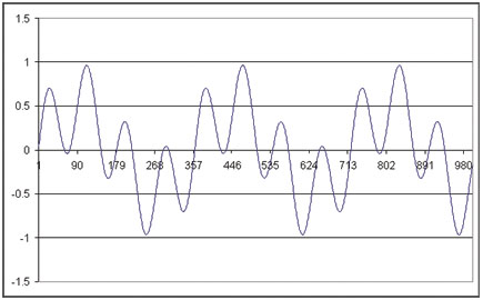
Introduction Neural networks have been applied to time-series prediction for many years from forecasting stock prices and sunspot activity to predicting the growth of tree rings. In essence all forms of time series prediction are fundamentally the same. Namely given data x=x(τ) which varies as a function of time τ, it should be possible to learn the function that maps xτ+1= xτ. Feed-forward networks can be applied directly to problems of this form provided the data is suitably pre-processed (in fact pre-processing of input data from any domain is always a very worthwhile effort be it feature extraction, dimensional reduction or outlier rejection etc.). Consider a single variable x which varies with time, one common approach is to sample x at regular time intervals to yield a series of observations xτ-2, xτ-1, xτ and so on. We can then take such observations and present them as the input vector to the network and use observation xτ+1 as the target value. By stepping along the time axis one sample at a time we can form the training set for the problem. In other words ‘given the last three samples what is the next value?’. Once we have trained the network we should then be able to present a new vector x'τ-2, x'τ-1, x'τ vector and predict x'τ+1. This is termed one step ahead prediction. We could also use the predicted value as part of the next input vector then depending on how many predicted values we allow to be fed back into the network we then have what is termed multi-step ahead prediction. Unfortunately the latter approach tends to diverge rapidly from the true pattern due to the accumulation of errors. There are a few problems with this simple approach though. First is the sampling rate between observations often requires empirical optimization. Secondly the time series may have an underlying trend, for example a steadily increasing value. If this is not removed via de-trending when the network is shown new data it may have great difficulty to extrapolate this trend. A more serious limitation is the implicit assumption that the statistical properties of the data generator are time dependant. If the generator is not time dependant then online learning methods have too be employed so the network can ‘track time’ in other words track the changing statistical properties of the generator. However, we wont worry about these issues yet as this is a beginners tutorial. Also we will not be covering training and testing issues, though they will be mentioned in passing. All we will be concentrating on is minimising the error during training of the network and looking at the sampling and network topology aspects of the neural networks. Introducing the problem. We will be using two basic data sets in this tutorial both artificially created so we do not have to de-trend them and we know the statistical properties of the generator are time dependant. The first a simple sine wave; the second is a supposition of two sine waves. These are shown in the figures below. So very simple signals both absolutely deterministic with no noise and from a bounded problem space. Or are they that simple? If you imagine walking along the simple sine wave, as you reach a peak (the slope decreases negatively) you know you will go down in a little while. Equally as you reach a dip (the slope decreases positively) you know you should go up in a bit. Also depending on how accurately you have measured the slope you also know how far along you are. But how accurately and for how long should you remember the slope for? The last 5 steps, 15, 30, 90 steps? It is even worse for the supposition of the sine waves! The local slope at each peak and trough are the same, but the peaks and troughs are at differing heights! Imagine standing on the peak at 100°? You know you should go down, but how far? If you where standing on the peak at 180° you still have to go down, but this time you go down further ‘absolute’ as you started this time at +0.3 but at the 100° peak you where at +1. The relative distance is still the same, but the absolute starting height is different! Remember you cannot cheat and look at the graph you only know where you have ‘just’ come from (this is similar to the local minima problem in neural net training) . In other words you can only look at the last ‘n’ samples you have. You could just remember every step you have ever taken but that’s cheating! This is why we said earlier that the sampling frequency for the training set requires ‘empirical’ optimisation! There are methods for helping us out but these are advanced methods from digital signal processing (DSP), dynamical systems theory (DST) and information theory and are way beyond the scope of this tutorial. So we have to work out a sampling frequency and a size of memory. Returning to the hill walking analogy we could remember every of the last five steps or every fifth step of the last 25. So what is the solution? Well we will just have to try some training sets empirically and see what happens. Remember the ‘memory’ is an input vector to the network, so that defines the number of input nodes of the network. We will term the ‘frequency’ as how often we remember a step. So for example we will remember every fifth step and keep a running note of the last twenty. In other words we will have walked 100 steps, but only remember the 1st, 6th, 11th so on. As you can imagine the number of possibilities grows astronomically large very quickly. Using this ‘wordy’ notation the training sets that we will be using are described in the table below.
We will not be using all of these training sets, but they are provided for you to experiment with. You may well get even better results than presented here. This is not an exhaustive paper on this subject but just a primer to get you going and to think about things. There are also many openly available papers on the internet for you to look through. There is also a program contained in the tutorial distribution pack to allow you to generate your own data sets (generateTrainingSets.java) please feel free to experiment with this and generate your own data sets. Why not extend it to add some ‘noise’ into the data, maybe even add some random errors in? Remember you will have to scale your network inputs accordingly between [-1...1] though. In fact why not change it to scale between [0...1] and using the Sigmoidal transfer function. Does this make the training any better? Introducing the Network. We will be using a standard multi layer back-propogation network often called a mult-layer perceptron (MLP). We will also use the hyperbolic tangent or TanH transfer functions as this has a range [-1…1] which fits our problem data nicely. We will not be changing the learning parameter or the momentum term either at the moment. We will just experiment with data sampling rates and differing topologies. Our next problem is what should the topology of the network be? Firstly the input layer is easily defined to be the memory size. Remember, we show the network a snapshot of where we have just been. Also we are only making a ‘one step ahead’ prediction network so we only need one output node. That just leaves the number of hidden nodes. Now there is some deep maths than we can use to help us predict the number of nodes and topology we will need in the hidden layers. One I will mention is a ‘rule of thumb’ called the Baum-Haussler rule. This states that;
Where Nhidden is the number of hidden nodes, Ntrain is the number of training patterns, Etolerance is the error we desire of the network, Ninput and Noutput are the number of input and output nodes respectively. This rule of thumb generally ensures that the network generalises rather than memorises the problem. It is relatively easy too make a neural network learn a problem perfectly. However, we don’t just want it to learn a given problem, we want it too be able to generalise the solution to data it has never seen before. Learning the problem perfectly but not being able to predict on data it has never been shown before is called over-fitting. The number of nodes is directly related to this balancing act between learning the problem but not generalising, and conversely not even learning the problem. This is why the number and topology of the nodes should be considered. But as this is a beginners guide we will ignore this, and anyway it is much more fun to play with the networks than follow a recipe! So what we will do is try some topologies out i.e. vary the number of hidden nodes and vary the number of hidden layers. Experimenting with the basic Sine wave. Let us start simply shall we? Using Neuroph create a network with 5 input nodes, 10 hidden nodes and 1 output node. So choose Networks->Multi Layer Perceptron. In the neurons num type 5 10 1 and choose Tanh as the transfer function. You will get a network that looks like this.
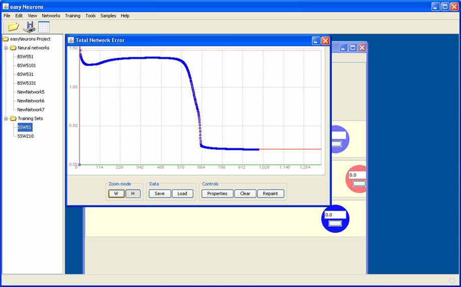
Now load the BSW51 training set. Do this by Training->New Training Set. Enter the name e.g. BSW51, type Supervised, inputs 5, outputs 1 and click next. Choose load from file and select the BSW51 training file and set the delimiter to be the Tab character. Remember a training set can be used over numerous network topologies just as long as the number of inputs and outputs matches the training set vector. Okay so let us train the network. Click the Train button the only parameter to change is the Limit Max Iterations so set this too be 1000. Click train and watch what happens. You should see something similar to the following.
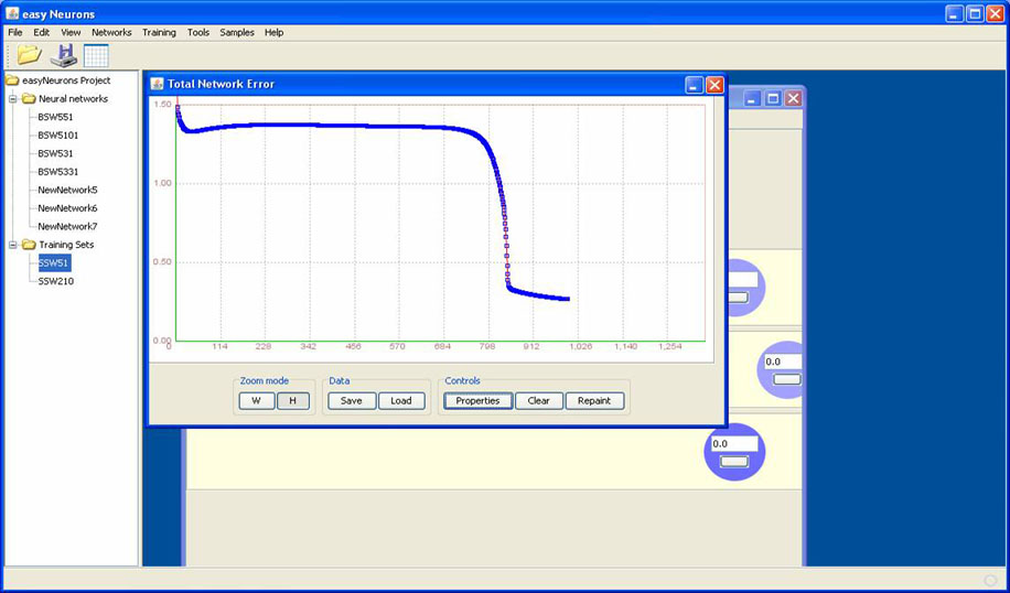
I say similar as depending on the initial weights connecting the neurones the error curve will vary. For example, all I did for the following example run was randomize the weights and re-run the training again. No other changes at all.
The behaviour is the same but we really start too minimise 100 iterations later. But note what happens we do not minimize the problem accurately enough, hence why we limited the number of iterations to 1000. It is always good practice to limit the number of iterations just to avoid a run-away system. Okay next change the topology and see what happens. So create a new network with 3 hidden nodes. Train this new network using the same data set (BSW51) and don’t change any learning parameters, just the maximum iterations to 1000. You should get something similar to the following.
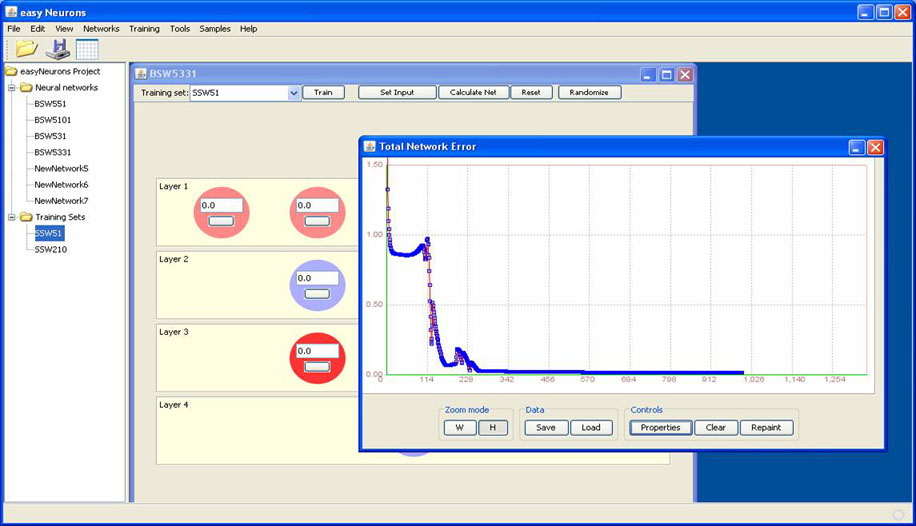
That is better we are converging much faster but still not getting the accuracy we want. We can change the number of hidden nodes, but something does not seem correct. The error curve just gets stretched or squashed and never really learns the problem accurately. What are our options? We could alter training parameters etc. but let us try a much simpler option first. Why not try a network with two hidden layers? Create a 5-3-3-1 network as you have done before. Then train it on the same data set. You should get something like the following.
That is much better, fast convergence and a much lower total network error. Remember we have not changed any training parameters simply the network topology. Experiment and see what happens. Does adding more nodes help or more layers? What is happening? Try it out. Remember building a neural network is a balancing act between the data, the number and topology of nodes and the training algorithm employed. All are mathematically tractable issues; just the mathematics can get a bit scary at times. Okay so far we have only changed the topology but remember one major issue in time-series prediction is the sampling of the data. So let us try that now. Load the training set BSW210. Make a network just as before but this time its topology is 10-3-3-1 and train it. Don’t change the parameters, just set the max iterations to 1000. When I run it I get the following.
This is much better. Fast convergence in fact the network stops training in 215 iterations with a total network error of <0.01. All we did was change the sampling frequency and how many steps we remembered. This is how important sampling frequency can be in time-series prediction. Remember this is a very simple sine wave, with no errors, noise, missing data etc. In fact it could not get much simpler. This neatly brings us onto the supposition sine wave example. I will only do one example just to prove it can be done, but you should really try them out for yourselves.
I have kept the topology and sampling i.e. data set secret. So try it out yourself, have a play, and scratch your head. A little hint is do not always look at your feet when you walk on a mountain, you will miss the big picture. Equally, don’t look to far ahead or you may trip up. Conclusions Sampling data correctly and choosing the correct network topology can have huge effects on time-series prediction. We have also seen how sometimes it is more important to have a couple of hidden layers with a few nodes rather than lots of nodes on one hidden layer. Neural net research and use is based in maths and statistics, but playing with them and trying them out is still the best bit. Well in my opinion anyway! Authors Notes Firstly I hope I have not bored you and you have enjoyed playing with Neuroph and this little tutorial. It is a very simple tutorial using a purely feed-forward network from the standard Neuroph toolkit. I hope in the future to develop further architectures to support time series modelling. Currently I am thinking about the following architectures; Time Delay NN, Jordan nets and Elman nets; plus a few bells and whistles such as convolutional memory, exponential trace memory and recurrent back-propogation. In addition I would like to develop some pre-processing libraries too clean the data up. Also there is a whole field of research regarding phase-space projection and false neighbour removal, to analyse the data, and to help predict what the memory size should be and also how often the data should be sampled. You can try all examples from this tutorial with online demo application or you can get all the materials from downloads section below. All comments and criticism are most appreciated and well received. DOWNLOADS 1. Neuroph framework with easyNeurons application See also:
|
||||||||||||||||||||||||||||||||||||||||||||||||||||||||


